
Recurrent Neural Networks (RNNs) are powerful sequence processing models that can handle data with temporal relationships. Unlike traditional feedforward neural networks, RNNs have connections that form directed cycles, allowing them to maintain memory of previous inputs. This makes them particularly effective for tasks involving sequential data like text, speech, time series, and more.
In this blog, we’ll explore different RNN architectures based on their input-output relationships, along with practical examples and implementations for each type.
Table of Contents
- One-to-One RNNs
- One-to-Many RNNs
- Many-to-One RNNs
- Many-to-Many RNNs (Synchronized)
- Many-to-Many RNNs (Encoder-Decoder)
- Advanced RNN Architectures
One-to-One RNNs
Architecture
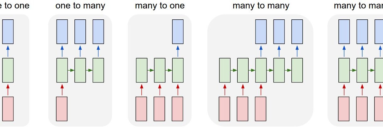
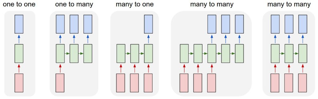
One-to-One RNNs are the simplest form and technically not recurrent at all. They take a single input and produce a single output, much like a standard feedforward neural network.
Input(x) → Neural Network → Output(y)
Example Use Case
Image classification, where a single image is classified into a single category.
Implementation
import torch
import torch.nn as nn

class SimpleNN(nn.Module):
    def __init__(self, input_size, hidden_size, output_size):
        super(SimpleNN, self).__init__()
        self.layer1 = nn.Linear(input_size, hidden_size)
        self.relu = nn.ReLU()
        self.layer2 = nn.Linear(hidden_size, output_size)

    def forward(self, x):
        out = self.layer1(x)
        out = self.relu(out)
        out = self.layer2(out)
        return out

# Example usage
input_size = 784  # For MNIST
hidden_size = 128
output_size = 10  # 10 digits

model = SimpleNN(input_size, hidden_size, output_size)

# For a single input
x = torch.randn(1, input_size)
output = model(x)
print(output.shape)  # torch.Size([1, 10])
Explanation
This isn’t truly an RNN since it lacks recurrence, but it’s included as a baseline for comparison. The model takes a flattened image (784 pixels for MNIST) and outputs probabilities for 10 digit classes.
One-to-Many RNNs
Architecture
One-to-Many RNNs take a single input and produce a sequence of outputs. The input is processed once, and then the network generates a series of outputs recursively.
Single Input(x) → RNN → Output sequence(y₁, y₂, ..., yₙ)
Example Use Case
Image captioning, where a single image generates a sequence of words describing it.
Implementation
import torch
import torch.nn as nn

class ImageCaptioningRNN(nn.Module):
    def __init__(self, image_feature_size, hidden_size, vocab_size, seq_length):
        super(ImageCaptioningRNN, self).__init__()
        self.hidden_size = hidden_size
        self.seq_length = seq_length

        # Image feature to hidden state
        self.image_to_hidden = nn.Linear(image_feature_size, hidden_size)

        # RNN cell (using GRU for simplicity)
        self.rnn_cell = nn.GRUCell(hidden_size, hidden_size)

        # Output layer
        self.hidden_to_output = nn.Linear(hidden_size, vocab_size)

    def forward(self, image_features):
        batch_size = image_features.size(0)

        # Initialize hidden state from image features
        hidden = self.image_to_hidden(image_features)

        # Container for outputs
        outputs = []

        # Input for first step is the hidden state
        input_t = hidden

        # Generate sequence
        for t in range(self.seq_length):
            # Update hidden state
            hidden = self.rnn_cell(input_t, hidden)

            # Generate output for this timestep
            output = self.hidden_to_output(hidden)
            outputs.append(output)

            # Next input is the current hidden state
            input_t = hidden

        # Stack outputs along sequence dimension
        outputs = torch.stack(outputs, dim=1)
        return outputs

# Example usage
image_feature_size = 2048  # From a CNN like ResNet
hidden_size = 512
vocab_size = 10000
seq_length = 20  # Maximum caption length

model = ImageCaptioningRNN(image_feature_size, hidden_size, vocab_size, seq_length)

# For a batch of images
image_features = torch.randn(32, image_feature_size)
captions = model(image_features)
print(captions.shape)  # torch.Size([32, 20, 10000])
Explanation
This RNN uses a single image input to generate a sequence of words. After processing the image features to create an initial hidden state, the model recursively generates each word based on the previous hidden state. At each step, the output is a probability distribution over the vocabulary.
Many-to-One RNNs
Architecture
Many-to-One RNNs process a sequence of inputs and produce a single output, typically at the end of the sequence.
Input sequence(x₁, x₂, ..., xₙ) → RNN → Single Output(y)
Example Use Case
Sentiment analysis of text, where a sequence of words is classified as positive or negative.
Implementation
import torch
import torch.nn as nn

class SentimentRNN(nn.Module):
    def __init__(self, vocab_size, embedding_dim, hidden_size, output_size):
        super(SentimentRNN, self).__init__()
        self.hidden_size = hidden_size

        # Word embeddings
        self.embedding = nn.Embedding(vocab_size, embedding_dim)

        # RNN layer
        self.rnn = nn.GRU(embedding_dim, hidden_size, batch_first=True)

        # Output layer
        self.fc = nn.Linear(hidden_size, output_size)

    def forward(self, x):
        # x shape: (batch_size, sequence_length)

        # Embed the input sequence
        x = self.embedding(x)  # (batch_size, sequence_length, embedding_dim)

        # Process through RNN
        _, hidden = self.rnn(x)  # hidden: (1, batch_size, hidden_size)

        # Use the final hidden state
        hidden = hidden.squeeze(0)  # (batch_size, hidden_size)

        # Pass through output layer
        output = self.fc(hidden)  # (batch_size, output_size)

        return output

# Example usage
vocab_size = 20000
embedding_dim = 300
hidden_size = 256
output_size = 2  # Binary sentiment (positive/negative)

model = SentimentRNN(vocab_size, embedding_dim, hidden_size, output_size)

# For a batch of sequences
batch_size = 64
sequence_length = 100
input_sequences = torch.randint(0, vocab_size, (batch_size, sequence_length))
sentiment = model(input_sequences)
print(sentiment.shape)  # torch.Size([64, 2])
Explanation
This model processes a sequence of word indices, embeds them, and passes them through a GRU layer. Only the final hidden state is used to make the prediction, which is then passed through a linear layer to get the sentiment classification.
Many-to-Many RNNs (Synchronized)
Architecture
In synchronized Many-to-Many RNNs, there’s an output for each input at the same time step.
Input sequence(x₁, x₂, ..., xₙ) → RNN → Output sequence(y₁, y₂, ..., yₙ)
Example Use Case
Part-of-speech tagging, where each word in a sentence is tagged with its grammatical role.
Implementation
import torch
import torch.nn as nn

class POSTaggerRNN(nn.Module):
    def __init__(self, vocab_size, embedding_dim, hidden_size, num_tags):
        super(POSTaggerRNN, self).__init__()

        # Word embeddings
        self.embedding = nn.Embedding(vocab_size, embedding_dim)

        # Bidirectional RNN for better context
        self.rnn = nn.LSTM(embedding_dim, hidden_size, batch_first=True, bidirectional=True)

        # Output layer (accounting for bidirectionality)
        self.fc = nn.Linear(hidden_size * 2, num_tags)

    def forward(self, x):
        # x shape: (batch_size, sequence_length)

        # Embed the input sequence
        x = self.embedding(x)  # (batch_size, sequence_length, embedding_dim)

        # Process through RNN
        outputs, _ = self.rnn(x)  # outputs: (batch_size, sequence_length, hidden_size*2)

        # Pass each output through the final layer
        tag_space = self.fc(outputs)  # (batch_size, sequence_length, num_tags)

        return tag_space

# Example usage
vocab_size = 20000
embedding_dim = 300
hidden_size = 256
num_tags = 45  # Number of POS tags

model = POSTaggerRNN(vocab_size, embedding_dim, hidden_size, num_tags)

# For a batch of sequences
batch_size = 32
sequence_length = 50
input_sequences = torch.randint(0, vocab_size, (batch_size, sequence_length))
pos_tags = model(input_sequences)
print(pos_tags.shape)  # torch.Size([32, 50, 45])
Explanation
This bidirectional LSTM processes a sequence of words and outputs a tag prediction for each word in the sequence. The model embeds each word, processes the entire sequence with a bidirectional LSTM to capture context in both directions, and then maps each hidden state to a tag probability distribution.
Many-to-Many RNNs (Encoder-Decoder)
Architecture
The encoder-decoder architecture first processes the entire input sequence (encoder) and then generates an output sequence (decoder), possibly of different length.
Input sequence(x₁, x₂, ..., xₙ) → Encoder → [State] → Decoder → Output sequence(y₁, y₂, ..., yₘ)
Example Use Case
Machine translation, where a sentence in one language is translated to another language.
Implementation
import torch
import torch.nn as nn
import torch.nn.functional as F

class Encoder(nn.Module):
    def __init__(self, input_vocab_size, embedding_dim, hidden_size):
        super(Encoder, self).__init__()
        self.hidden_size = hidden_size

        self.embedding = nn.Embedding(input_vocab_size, embedding_dim)
        self.lstm = nn.LSTM(embedding_dim, hidden_size, batch_first=True)

    def forward(self, x):
        # x shape: (batch_size, sequence_length)

        embedded = self.embedding(x)  # (batch_size, sequence_length, embedding_dim)
        outputs, (hidden, cell) = self.lstm(embedded)

        return outputs, hidden, cell

class Decoder(nn.Module):
    def __init__(self, output_vocab_size, embedding_dim, hidden_size):
        super(Decoder, self).__init__()
        self.hidden_size = hidden_size

        self.embedding = nn.Embedding(output_vocab_size, embedding_dim)
        self.lstm = nn.LSTM(embedding_dim, hidden_size, batch_first=True)
        self.fc = nn.Linear(hidden_size, output_vocab_size)

    def forward(self, x, hidden, cell):
        # x shape: (batch_size, 1)

        embedded = self.embedding(x)  # (batch_size, 1, embedding_dim)

        output, (hidden, cell) = self.lstm(embedded, (hidden, cell))
        # output: (batch_size, 1, hidden_size)

        prediction = self.fc(output.squeeze(1))  # (batch_size, output_vocab_size)

        return prediction, hidden, cell

class Seq2Seq(nn.Module):
    def __init__(self, encoder, decoder, device):
        super(Seq2Seq, self).__init__()
        self.encoder = encoder
        self.decoder = decoder
        self.device = device

    def forward(self, source, target, teacher_forcing_ratio=0.5):
        # source: (batch_size, source_length)
        # target: (batch_size, target_length)

        batch_size = source.shape[0]
        target_length = target.shape[1]
        target_vocab_size = self.decoder.fc.out_features

        # Tensor to store decoder outputs
        outputs = torch.zeros(batch_size, target_length, target_vocab_size).to(self.device)

        # Encode the source sequence
        _, hidden, cell = self.encoder(source)

        # First decoder input is the <SOS> token
        decoder_input = target[:, 0].unsqueeze(1)  # (batch_size, 1)

        for t in range(1, target_length):
            # Pass through decoder
            output, hidden, cell = self.decoder(decoder_input, hidden, cell)

            # Store prediction
            outputs[:, t, :] = output

            # Decide whether to use teacher forcing
            teacher_force = torch.rand(1).item() < teacher_forcing_ratio

            # Get the highest predicted token
            top1 = output.argmax(1)

            # Use either prediction or actual target as next input
            decoder_input = target[:, t].unsqueeze(1) if teacher_force else top1.unsqueeze(1)

        return outputs

# Example usage
input_vocab_size = 10000
output_vocab_size = 8000
embedding_dim = 256
hidden_size = 512
device = torch.device('cuda' if torch.cuda.is_available() else 'cpu')

encoder = Encoder(input_vocab_size, embedding_dim, hidden_size).to(device)
decoder = Decoder(output_vocab_size, embedding_dim, hidden_size).to(device)
model = Seq2Seq(encoder, decoder, device).to(device)

# For a batch of sequences
batch_size = 16
source_length = 20
target_length = 25
source = torch.randint(0, input_vocab_size, (batch_size, source_length)).to(device)
target = torch.randint(0, output_vocab_size, (batch_size, target_length)).to(device)

output = model(source, target)
print(output.shape)  # torch.Size([16, 25, 8000])
Explanation
This is a more complex sequence-to-sequence model with an encoder-decoder architecture. The encoder processes the entire input sequence and passes its final state to the decoder, which then generates an output sequence. The implementation includes teacher forcing, where during training the model sometimes uses the true target from the previous time step instead of its own prediction.
Advanced RNN Architectures
While the basic types above cover the fundamental input-output relationships, modern RNN applications often use more advanced architectures:
LSTM (Long Short-Term Memory)
LSTMs address the vanishing gradient problem in standard RNNs with a more complex cell structure that includes input, forget, and output gates.
GRU (Gated Recurrent Unit)
GRUs are a simplified version of LSTMs with fewer parameters but similar capabilities for long-term dependency modeling.
Bidirectional RNNs
These process sequences in both forward and backward directions to capture context from both past and future time steps.
Attention Mechanisms
Attention allows models to focus on relevant parts of the input sequence when generating each output element, significantly improving performance for tasks like translation.
Transformers
While not traditional RNNs, transformers have largely replaced RNNs in many sequence processing tasks due to their parallelization capabilities and stronger performance.
Conclusion
Recurrent Neural Networks offer versatile architectures for processing sequential data across various applications. From the simple one-to-many models for image captioning to the complex encoder-decoder structures for machine translation, RNNs and their variants enable powerful modeling of temporal dependencies.
Understanding the different input-output relationships in RNN architectures is crucial for selecting the right approach for your specific sequence processing task. While traditional RNNs have been widely used, more advanced architectures like LSTMs, GRUs, and attention-based models have pushed the boundaries of sequence modeling even further.