I specialize in the dynamic and ever-evolving field of Artificial Intelligence, Data Science. My expertise lies in harnessing the power of AI, Natural Language Processing (NLP), Data Engineering, and cutting-edge AI-ML technologies to unravel complex problems and unlock new possibilities.
Inventions sparks curiosity, Leading to a continuous cycle of exploration and advancement.
Hi, I’m Tejas kamble a Data EngineerAI EngineerResearcher
I specialize in the dynamic and ever-evolving field of Artificial Intelligence, Data Science. My expertise lies in harnessing the power of AI, Natural Language Processing (NLP), Data Engineering, and cutting-edge AI-ML technologies to unravel complex problems and unlock new possibilities.
find with me
best skill on
Visit my portfolio & Hire me
About Me
With a passion for creating intelligent systems, I thrive on developing innovative solutions that bridge the gap between raw data and actionable insights. Whether it’s crafting robust algorithms, engineering data pipelines, or delving into the realms of machine learning, I am dedicated to pushing the boundaries of what AI can achieve.
I’ve actively engaged in developing AI-driven applications, collaborating on research initiatives, and contributing to the advancement of the field. My current endeavors include spearheading two significant projects – one focused on exploring the intersection of AI and healthcare, and another involving the development of a platform that seamlessly integrates AI into everyday life.
Cloud cost management has evolved from manual spreadsheet tracking to sophisticated AI-driven automation. As organizations increasingly adopt multi-cloud strategies, the complexity of cost optimization grows exponentially. This comprehensive guide explores building agentic AI systems that autonomously manage cloud costs, leveraging open-source models and cutting-edge AI frameworks.
Understanding Agentic AI Systems
Agentic AI systems represent a paradigm shift from traditional reactive AI to proactive, goal-oriented artificial intelligence. Unlike conventional AI models that respond to queries, agentic systems operate autonomously, making decisions and taking actions to achieve specific objectives.
Core Characteristics of Agentic AI
Autonomy: The system operates independently, making decisions without constant human intervention while respecting predefined boundaries and policies.
Goal-Oriented Behavior: Each agent has clear objectives, such as minimizing cloud costs while maintaining performance SLAs, and continuously works toward achieving these goals.
Environmental Awareness: Agents continuously monitor their environment, understanding cloud resource utilization, cost trends, and performance metrics in real-time.
Learning and Adaptation: The system learns from past decisions, improving its cost optimization strategies over time through reinforcement learning and feedback loops.
Multi-Agent Coordination: Different specialized agents collaborate, such as a cost monitoring agent working with a resource optimization agent and a compliance agent.
Architecture of Agentic AI for Cloud Cost Management
Multi-Agent System Design
The architecture consists of specialized agents, each responsible for specific aspects of cloud cost management:
Cost Monitoring Agent: Continuously collects and analyzes billing data from multiple cloud providers, detecting anomalies and trends in real-time.
Resource Optimization Agent: Evaluates resource utilization patterns and makes recommendations or autonomous decisions about rightsizing, scaling, and resource allocation.
Compliance Agent: Ensures all cost optimization actions comply with organizational policies, regulatory requirements, and client-specific constraints.
Forecasting Agent: Uses predictive models to anticipate future costs and resource needs, enabling proactive optimization strategies.
Notification Agent: Manages communication with stakeholders, sending alerts, reports, and recommendations through appropriate channels.
Action Execution Agent: Safely implements approved optimization actions across cloud environments, with rollback capabilities for safety.
Data Flow and Integration Layer
The system integrates with multiple data sources and APIs:
Cloud Provider APIs: Direct integration with AWS Cost Explorer, Azure Cost Management, Google Cloud Billing, and other cloud providers’ cost and usage APIs.
Infrastructure Monitoring: Integration with Prometheus, Grafana, Datadog, or New Relic for real-time performance metrics.
Configuration Management: Connection to Terraform, Ansible, or CloudFormation for infrastructure state management.
Business Systems: Integration with ERP, CRM, and project management systems for cost allocation and chargeback functionality.
Open Source AI Models and Frameworks
Large Language Models Integration
Ollama Integration: Ollama provides local deployment of open-source models, ensuring data privacy and reducing API costs. Key models include:
Llama 2/3: Excellent for natural language processing tasks, generating cost optimization reports, and explaining complex cost patterns to stakeholders
Code Llama: Specialized for generating and analyzing infrastructure code, automating Terraform configurations, and creating cost optimization scripts
Mistral 7B/8x7B: Efficient models for real-time decision making and cost analysis with lower computational requirements
Anthropic Claude Integration: While not open-source, Claude’s API provides sophisticated reasoning capabilities for complex cost optimization scenarios and policy interpretation.
Mistral AI Models: Open-weight models offering excellent performance for cost analysis tasks:
Mixtral 8x7B: Mixture of experts model providing efficient processing for multi-task cost optimization
Mistral 7B: Compact model suitable for edge deployment and real-time decision making
Specialized AI Tools and Libraries
Machine Learning Frameworks:
scikit-learn: For traditional ML tasks like anomaly detection, clustering cost patterns, and regression analysis
XGBoost/LightGBM: Gradient boosting for accurate cost forecasting and resource usage prediction
PyTorch/TensorFlow: Deep learning frameworks for complex pattern recognition in cost data
Time Series Analysis:
Prophet: Facebook’s time series forecasting tool, excellent for predicting cloud costs with seasonal patterns
ARIMA/SARIMA: Classical time series models for cost trend analysis
Neural Prophet: Deep learning approach to time series forecasting
Reinforcement Learning:
Stable Baselines3: Implementation of RL algorithms for autonomous cost optimization decisions
Ray RLlib: Distributed reinforcement learning for complex multi-agent scenarios
Natural Language Processing:
Transformers (Hugging Face): Pre-trained models for processing cost reports, policy documents, and generating explanations
spaCy: Efficient NLP library for text processing and entity extraction from cost documentation
Technical Implementation Stack
Backend Infrastructure
Core Application Framework:
# FastAPI-based microservices architecture
from fastapi import FastAPI, BackgroundTasks
from pydantic import BaseModel
import asyncio
from typing import List, Dict
import httpx

app = FastAPI(title="Agentic Cloud Cost Management")

class CostAgent:
    def __init__(self, model_endpoint: str):
        self.model_endpoint = model_endpoint
        self.client = httpx.AsyncClient()

    async def analyze_costs(self, cost_data: Dict):
        # Integration with Ollama or other model endpoints
        pass
Message Queue and Orchestration:
Apache Kafka: Real-time data streaming for cost events and optimization triggers
Celery with Redis: Task queue for asynchronous cost optimization jobs
Apache Airflow: Workflow orchestration for complex cost management pipelines
Database Architecture:
InfluxDB: Time-series database for storing cost and usage metrics
PostgreSQL: Relational database for client configurations, policies, and audit trails
MongoDB: Document store for unstructured data like cost reports and optimization recommendations
Redis: Caching layer for frequently accessed cost data and model predictions
Terraform Provider: Custom provider for cost-optimized resource provisioning
Pulumi: Modern IaC with native programming language support
CDK (Cloud Development Kit): Define cloud resources using familiar programming languages
Agent Communication and Coordination
Inter-Agent Communication Protocol
Message Passing System:
from dataclasses import dataclass
from enum import Enum
from typing import Any, Dict

class MessageType(Enum):
    COST_ALERT = "cost_alert"
    OPTIMIZATION_REQUEST = "optimization_request"
    ACTION_APPROVAL = "action_approval"
    STATUS_UPDATE = "status_update"

@dataclass
class AgentMessage:
    sender: str
    recipient: str
    message_type: MessageType
    payload: Dict[str, Any]
    timestamp: float
    priority: int = 1

class AgentCommunicationHub:
    def __init__(self):
        self.agents = {}
        self.message_queue = asyncio.Queue()

    async def route_message(self, message: AgentMessage):
        if message.recipient in self.agents:
            await self.agents[message.recipient].receive_message(message)
Consensus Mechanisms: Implement voting systems for critical decisions affecting multiple clients or significant cost impacts, ensuring no single agent can make potentially harmful decisions without consensus.
Event-Driven Architecture
Event Streaming with Kafka:
from kafka import KafkaProducer, KafkaConsumer
import json

class CostEventProducer:
    def __init__(self):
        self.producer = KafkaProducer(
            bootstrap_servers=['localhost:9092'],
            value_serializer=lambda x: json.dumps(x).encode('utf-8')
        )

    def emit_cost_event(self, event_type: str, data: Dict):
        event = {
            'event_type': event_type,
            'timestamp': time.time(),
            'data': data
        }
        self.producer.send('cost-events', event)

class OptimizationAgent:
    def __init__(self):
        self.consumer = KafkaConsumer(
            'cost-events',
            bootstrap_servers=['localhost:9092'],
            auto_offset_reset='latest',
            value_deserializer=lambda m: json.loads(m.decode('utf-8'))
        )

    async def process_events(self):
        for message in self.consumer:
            await self.handle_cost_event(message.value)
Implementing Intelligent Cost Optimization
Anomaly Detection System
Statistical Anomaly Detection:
import numpy as np
from sklearn.ensemble import IsolationForest
from sklearn.preprocessing import StandardScaler

class CostAnomalyDetector:
    def __init__(self):
        self.model = IsolationForest(contamination=0.1, random_state=42)
        self.scaler = StandardScaler()
        self.is_trained = False

    def train(self, historical_costs: np.ndarray):
        scaled_costs = self.scaler.fit_transform(historical_costs)
        self.model.fit(scaled_costs)
        self.is_trained = True

    def detect_anomalies(self, current_costs: np.ndarray) -> List[bool]:
        if not self.is_trained:
            raise ValueError("Model must be trained first")

        scaled_costs = self.scaler.transform(current_costs)
        anomaly_scores = self.model.decision_function(scaled_costs)
        return self.model.predict(scaled_costs) == -1
Deep Learning Anomaly Detection:
import torch
import torch.nn as nn
from torch.utils.data import DataLoader, TensorDataset

class CostAutoencoderAnomalyDetector(nn.Module):
    def __init__(self, input_dim: int, hidden_dims: List[int]):
        super().__init__()

        # Encoder
        encoder_layers = []
        current_dim = input_dim
        for hidden_dim in hidden_dims:
            encoder_layers.extend([
                nn.Linear(current_dim, hidden_dim),
                nn.ReLU(),
                nn.BatchNorm1d(hidden_dim)
            ])
            current_dim = hidden_dim

        # Decoder
        decoder_layers = []
        for i in range(len(hidden_dims) - 1, -1, -1):
            decoder_layers.extend([
                nn.Linear(current_dim, hidden_dims[i] if i > 0 else input_dim),
                nn.ReLU() if i > 0 else nn.Sigmoid()
            ])
            current_dim = hidden_dims[i] if i > 0 else input_dim

        self.encoder = nn.Sequential(*encoder_layers)
        self.decoder = nn.Sequential(*decoder_layers)

    def forward(self, x):
        encoded = self.encoder(x)
        decoded = self.decoder(encoded)
        return decoded
Predictive Cost Modeling
Time Series Forecasting with Neural Networks:
import pytorch_lightning as pl
from pytorch_forecasting import TimeSeriesDataSet, NBeats
import pandas as pd

class CostForecastingModel:
    def __init__(self):
        self.model = None
        self.training_data = None

    def prepare_data(self, cost_history: pd.DataFrame):
        # Convert cost history to time series format
        self.training_data = TimeSeriesDataSet(
            cost_history,
            time_idx="day",
            target="cost",
            group_ids=["client_id", "service"],
            min_encoder_length=30,
            max_encoder_length=90,
            min_prediction_length=7,
            max_prediction_length=30,
            static_categoricals=["client_id", "service"],
            time_varying_known_reals=["day_of_week", "month", "quarter"],
            time_varying_unknown_reals=["cost"],
        )

    def train_model(self):
        self.model = NBeats.from_dataset(
            self.training_data,
            learning_rate=3e-2,
            weight_decay=1e-8,
            widths=[32, 512],
            backcast_loss_ratio=1.0,
        )

        trainer = pl.Trainer(max_epochs=50, gpus=1)
        trainer.fit(self.model, self.training_data)
Multi-Tenant Architecture for Service Organizations
Client Isolation and Security
Tenant Management System:
from sqlalchemy import create_engine, Column, String, Integer, JSON, DateTime
from sqlalchemy.ext.declarative import declarative_base
from sqlalchemy.orm import sessionmaker
import hashlib
import secrets

Base = declarative_base()

class Tenant(Base):
    __tablename__ = 'tenants'

    id = Column(String, primary_key=True)
    name = Column(String, nullable=False)
    api_key_hash = Column(String, nullable=False)
    config = Column(JSON, default={})
    created_at = Column(DateTime)

    def generate_api_key(self):
        api_key = secrets.token_urlsafe(32)
        self.api_key_hash = hashlib.sha256(api_key.encode()).hexdigest()
        return api_key

class TenantManager:
    def __init__(self, database_url: str):
        self.engine = create_engine(database_url)
        self.SessionLocal = sessionmaker(bind=self.engine)

    def create_tenant(self, name: str, config: Dict) -> Tuple[str, str]:
        tenant = Tenant(
            id=secrets.token_urlsafe(16),
            name=name,
            config=config
        )
        api_key = tenant.generate_api_key()

        with self.SessionLocal() as session:
            session.add(tenant)
            session.commit()

        return tenant.id, api_key
Data Isolation with Row-Level Security:
-- PostgreSQL RLS for tenant data isolation
CREATE POLICY tenant_isolation ON cost_data
    FOR ALL TO application_role
    USING (tenant_id = current_setting('app.current_tenant'));

-- Function to set tenant context
CREATE OR REPLACE FUNCTION set_tenant_context(tenant_id TEXT)
RETURNS VOID AS $$
BEGIN
    PERFORM set_config('app.current_tenant', tenant_id, true);
END;
$$ LANGUAGE plpgsql;
from dataclasses import dataclass
from typing import List, Callable, Any
from enum import Enum

class PolicyType(Enum):
    COST_LIMIT = "cost_limit"
    RESOURCE_CONSTRAINT = "resource_constraint"
    APPROVAL_REQUIRED = "approval_required"
    COMPLIANCE_RULE = "compliance_rule"

@dataclass
class Policy:
    id: str
    name: str
    policy_type: PolicyType
    conditions: Dict[str, Any]
    actions: List[str]
    priority: int
    active: bool = True

class PolicyEngine:
    def __init__(self):
        self.policies: Dict[str, Policy] = {}
        self.rule_evaluators: Dict[PolicyType, Callable] = {
            PolicyType.COST_LIMIT: self._evaluate_cost_limit,
            PolicyType.RESOURCE_CONSTRAINT: self._evaluate_resource_constraint,
            PolicyType.APPROVAL_REQUIRED: self._evaluate_approval_requirement,
            PolicyType.COMPLIANCE_RULE: self._evaluate_compliance_rule
        }

    def add_policy(self, policy: Policy):
        self.policies[policy.id] = policy

    async def evaluate_action(self, action: Dict, context: Dict) -> Dict:
        """Evaluate if an action is allowed based on active policies"""
        evaluation_results = []

        # Sort policies by priority
        sorted_policies = sorted(
            [p for p in self.policies.values() if p.active],
            key=lambda x: x.priority,
            reverse=True
        )

        for policy in sorted_policies:
            evaluator = self.rule_evaluators.get(policy.policy_type)
            if evaluator:
                result = await evaluator(policy, action, context)
                evaluation_results.append({
                    'policy_id': policy.id,
                    'policy_name': policy.name,
                    'allowed': result['allowed'],
                    'reason': result['reason'],
                    'required_approvals': result.get('required_approvals', [])
                })

        # Determine final decision
        allowed = all(result['allowed'] for result in evaluation_results)
        required_approvals = []
        for result in evaluation_results:
            required_approvals.extend(result.get('required_approvals', []))

        return {
            'allowed': allowed,
            'policy_evaluations': evaluation_results,
            'required_approvals': list(set(required_approvals))
        }

    async def _evaluate_cost_limit(self, policy: Policy, action: Dict, context: Dict) -> Dict:
        current_cost = context.get('current_monthly_cost', 0)
        projected_cost = current_cost + action.get('cost_impact', 0)
        cost_limit = policy.conditions.get('monthly_limit', float('inf'))

        if projected_cost > cost_limit:
            return {
                'allowed': False,
                'reason': f"Action would exceed monthly cost limit of ${cost_limit:,.2f}"
            }

        return {'allowed': True, 'reason': 'Within cost limits'}

    async def _evaluate_resource_constraint(self, policy: Policy, action: Dict, context: Dict) -> Dict:
        # Implement resource constraint evaluation
        return {'allowed': True, 'reason': 'Resource constraints satisfied'}

    async def _evaluate_approval_requirement(self, policy: Policy, action: Dict, context: Dict) -> Dict:
        cost_impact = action.get('cost_impact', 0)
        approval_threshold = policy.conditions.get('cost_threshold', 1000)

        if abs(cost_impact) > approval_threshold:
            return {
                'allowed': False,
                'reason': f"Action requires approval (cost impact: ${cost_impact:,.2f})",
                'required_approvals': policy.conditions.get('approvers', ['manager'])
            }

        return {'allowed': True, 'reason': 'No approval required'}

    async def _evaluate_compliance_rule(self, policy: Policy, action: Dict, context: Dict) -> Dict:
        # Implement compliance rule evaluation (PCI, HIPAA, SOX, etc.)
        compliance_tags = context.get('compliance_tags', [])
        required_tags = policy.conditions.get('required_tags', [])

        if not all(tag in compliance_tags for tag in required_tags):
            return {
                'allowed': False,
                'reason': f"Missing required compliance tags: {set(required_tags) - set(compliance_tags)}"
            }

        return {'allowed': True, 'reason': 'Compliance requirements met'}
Advanced Model Integration Techniques
Hybrid Local-Cloud Model Architecture
Intelligent Model Selection:
class HybridModelOrchestrator:
    def __init__(self):
        self.local_models = {
            'ollama_llama3': 'http://localhost:11434/api/generate',
            'ollama_mistral': 'http://localhost:11434/api/generate',
            'ollama_codellama': 'http://localhost:11434/api/generate'
        }

        self.cloud_models = {
            'claude': 'https://api.anthropic.com/v1/messages',
            'mistral_large': 'https://api.mistral.ai/v1/chat/completions'
        }

        self.model_characteristics = {
            'ollama_llama3': {'latency': 'low', 'cost': 'free', 'privacy': 'high', 'capability': 'medium'},
            'ollama_mistral': {'latency': 'low', 'cost': 'free', 'privacy': 'high', 'capability': 'medium'},
            'claude': {'latency': 'medium', 'cost': 'medium', 'privacy': 'medium', 'capability': 'high'},
            'mistral_large': {'latency': 'medium', 'cost': 'low', 'privacy': 'medium', 'capability': 'high'}
        }

    async def select_optimal_model(self, task_type: str, requirements: Dict) -> str:
        """Select the best model based on task requirements"""

        # Define selection criteria
        if requirements.get('privacy_critical', False):
            # Use only local models for sensitive data
            candidates = list(self.local_models.keys())
        else:
            candidates = list(self.local_models.keys()) + list(self.cloud_models.keys())

        # Score models based on requirements
        scored_models = []
        for model in candidates:
            score = self._calculate_model_score(model, task_type, requirements)
            scored_models.append((model, score))

        # Return best scoring model
        return max(scored_models, key=lambda x: x[1])[0]

    def _calculate_model_score(self, model: str, task_type: str, requirements: Dict) -> float:
        characteristics = self.model_characteristics[model]
        score = 0.0

        # Latency scoring
        if requirements.get('max_latency', 10) < 2:
            score += 3 if characteristics['latency'] == 'low' else 0

        # Cost scoring
        if requirements.get('cost_sensitive', False):
            score += 2 if characteristics['cost'] == 'free' else 0

        # Privacy scoring
        if requirements.get('privacy_critical', False):
            score += 4 if characteristics['privacy'] == 'high' else 0

        # Capability scoring for complex tasks
        if task_type in ['complex_analysis', 'strategic_planning']:
            score += 3 if characteristics['capability'] == 'high' else 1

        return score

    async def execute_with_fallback(self, prompt: str, task_type: str, requirements: Dict) -> Dict:
        """Execute request with automatic fallback to alternative models"""

        primary_model = await self.select_optimal_model(task_type, requirements)

        try:
            return await self._query_model(primary_model, prompt)
        except Exception as e:
            # Fallback strategy
            fallback_models = [m for m in self.model_characteristics.keys() if m != primary_model]

            for fallback_model in fallback_models:
                try:
                    result = await self._query_model(fallback_model, prompt)
                    # Log fallback usage
                    self._log_fallback(primary_model, fallback_model, str(e))
                    return result
                except Exception:
                    continue

            raise Exception("All models failed")

    async def _query_model(self, model_name: str, prompt: str) -> Dict:
        if model_name in self.local_models:
            return await self._query_ollama(model_name, prompt)
        else:
            return await self._query_cloud_model(model_name, prompt)

    async def _query_ollama(self, model_name: str, prompt: str) -> Dict:
        model_key = model_name.split('_')[1]  # Extract model name (llama3, mistral, etc.)

        payload = {
            "model": model_key,
            "prompt": prompt,
            "stream": False,
            "options": {
                "temperature": 0.1,
                "top_p": 0.9,
                "num_predict": 512
            }
        }

        async with httpx.AsyncClient() as client:
            response = await client.post(
                self.local_models[model_name],
                json=payload,
                timeout=30.0
            )
            response.raise_for_status()
            return response.json()
Advanced Prompt Engineering for Cost Management
Domain-Specific Prompt Templates:
class CostManagementPrompts:
    def __init__(self):
        self.templates = {
            'anomaly_analysis': """
You are a cloud cost optimization expert. Analyze the following cost data and identify anomalies:

Cost Data:
{cost_data}

Context:
- Historical average: ${historical_avg}
- Current cost: ${current_cost}
- Time period: {time_period}
- Services involved: {services}

Please provide:
1. Anomaly detection (Yes/No) with confidence score
2. Root cause analysis
3. Recommended immediate actions
4. Potential cost impact if not addressed

Format your response as JSON with the following structure:
{{
    "anomaly_detected": boolean,
    "confidence_score": float,
    "root_cause": "string",
    "immediate_actions": ["action1", "action2"],
    "cost_impact": float,
    "reasoning": "detailed explanation"
}}
""",

            'optimization_recommendation': """
You are an expert cloud architect focused on cost optimization. Given the following resource utilization data, provide optimization recommendations:

Resource Data:
{resource_data}

Current Configuration:
{current_config}

Performance Requirements:
{performance_requirements}

Budget Constraints:
{budget_constraints}

Provide specific, actionable recommendations that:
1. Reduce costs while maintaining or improving performance
2. Consider business requirements and constraints
3. Include estimated cost savings
4. Prioritize recommendations by impact and effort

Format as JSON:
{{
    "recommendations": [
        {{
            "action": "string",
            "estimated_savings": float,
            "effort_level": "low|medium|high",
            "risk_level": "low|medium|high",
            "implementation_steps": ["step1", "step2"],
            "expected_timeline": "string"
        }}
    ],
    "total_potential_savings": float,
    "implementation_priority": ["rec1", "rec2", "rec3"]
}}
""",

            'executive_summary': """
Create an executive summary for cloud cost management based on the following data:

Financial Summary:
- Total monthly cost: ${total_cost}
- Month-over-month change: {mom_change}%
- Year-over-year change: {yoy_change}%
- Budget utilization: {budget_utilization}%

Key Metrics:
{key_metrics}

Optimization Actions Taken:
{actions_taken}

Upcoming Initiatives:
{upcoming_initiatives}

Write a professional executive summary that:
1. Highlights key financial performance
2. Explains significant changes
3. Summarizes optimization impact
4. Outlines strategic recommendations
5. Uses business-friendly language (avoid technical jargon)

Keep it concise (200-300 words) and focus on business value.
"""
        }

    def get_prompt(self, template_name: str, **kwargs) -> str:
        if template_name not in self.templates:
            raise ValueError(f"Template {template_name} not found")

        return self.templates[template_name].format(**kwargs)

    def create_chain_of_thought_prompt(self, base_prompt: str, thinking_steps: List[str]) -> str:
        """Create a chain-of-thought prompt for complex reasoning"""

        cot_prefix = """
Before providing your final answer, think through this step by step:

"""

        for i, step in enumerate(thinking_steps, 1):
            cot_prefix += f"{i}. {step}\n"

        cot_prefix += "\nNow, work through each step and provide your final answer:\n\n"

        return cot_prefix + base_prompt
Multi-Modal AI Integration
Integration with Vision Models for Infrastructure Diagrams:
class MultiModalCostAnalyzer:
    def __init__(self):
        self.vision_models = {
            'diagram_analysis': 'llava:latest',  # Ollama vision model
            'chart_interpretation': 'bakllava:latest'
        }

    async def analyze_architecture_diagram(self, image_path: str, cost_context: Dict) -> Dict:
        """Analyze infrastructure diagrams to identify cost optimization opportunities"""

        # Read image
        with open(image_path, 'rb') as img_file:
            image_data = base64.b64encode(img_file.read()).decode()

        prompt = f"""
Analyze this cloud architecture diagram and identify potential cost optimization opportunities.

Consider the following cost context:
- Current monthly spend: ${cost_context['monthly_spend']}
- Top cost drivers: {', '.join(cost_context['top_drivers'])}
- Performance requirements: {cost_context['performance_requirements']}

Look for:
1. Over-provisioned resources
2. Unnecessary redundancy
3. Inefficient data flow patterns
4. Missing cost optimization services
5. Opportunities for serverless migration

Provide specific, actionable recommendations with estimated cost impact.
"""

        # Query vision model through Ollama
        response = await self._query_vision_model('llava:latest', prompt, image_data)

        return {
            'diagram_analysis': response,
            'cost_optimization_score': self._calculate_optimization_score(response),
            'recommended_actions': self._extract_actions(response)
        }

    async def interpret_cost_charts(self, chart_images: List[str]) -> Dict:
        """Interpret cost trend charts and graphs"""

        interpretations = []

        for chart_path in chart_images:
            with open(chart_path, 'rb') as img_file:
                image_data = base64.b64encode(img_file.read()).decode()

            prompt = """
Analyze this cost chart/graph and provide insights:

1. Identify trends and patterns
2. Spot anomalies or unusual spikes
3. Determine seasonality effects
4. Suggest areas for investigation
5. Provide forecasting insights

Be specific about time periods, cost values, and percentage changes you observe.
"""

            interpretation = await self._query_vision_model('bakllava:latest', prompt, image_data)
            interpretations.append(interpretation)

        return {
            'chart_interpretations': interpretations,
            'combined_insights': await self._synthesize_chart_insights(interpretations)
        }

    async def _query_vision_model(self, model: str, prompt: str, image_data: str) -> str:
        payload = {
            "model": model,
            "prompt": prompt,
            "images": [image_data],
            "stream": False
        }

        async with httpx.AsyncClient() as client:
            response = await client.post(
                "http://localhost:11434/api/generate",
                json=payload,
                timeout=60.0
            )
            response.raise_for_status()
            return response.json()['response']
Performance Optimization and Scaling
Distributed Agent Architecture
Agent Cluster Management:
import asyncio
import aioredis
from typing import List, Dict, Any
from dataclasses import dataclass, asdict
from datetime import datetime, timedelta

@dataclass
class AgentNode:
    node_id: str
    agent_type: str
    status: str
    last_heartbeat: datetime
    current_load: float
    max_capacity: int
    client_assignments: List[str]

class DistributedAgentManager:
    def __init__(self, redis_url: str):
        self.redis_url = redis_url
        self.redis = None
        self.local_agents: Dict[str, Any] = {}
        self.node_id = secrets.token_urlsafe(8)

    async def initialize(self):
        self.redis = await aioredis.from_url(self.redis_url)
        await self.register_node()

        # Start background tasks
        asyncio.create_task(self.heartbeat_loop())
        asyncio.create_task(self.load_balancer_loop())

    async def register_node(self):
        """Register this node in the distributed cluster"""
        node_info = AgentNode(
            node_id=self.node_id,
            agent_type="multi_purpose",
            status="active",
            last_heartbeat=datetime.now(),
            current_load=0.0,
            max_capacity=100,
            client_assignments=[]
        )

        await self.redis.hset(
            "agent_nodes",
            self.node_id,
            json.dumps(asdict(node_info), default=str)
        )

    async def heartbeat_loop(self):
        """Send periodic heartbeats to maintain cluster membership"""
        while True:
            try:
                await self.redis.hset(
                    "agent_nodes",
                    self.node_id,
                    json.dumps({
                        "node_id": self.node_id,
                        "status": "active",
                        "last_heartbeat": datetime.now().isoformat(),
                        "current_load": self.calculate_current_load(),
                        "client_assignments": list(self.local_agents.keys())
                    })
                )
                await asyncio.sleep(30)  # Heartbeat every 30 seconds
            except Exception as e:
                print(f"Heartbeat error: {e}")
                await asyncio.sleep(5)

    async def distribute_work(self, task: Dict) -> str:
        """Distribute work to the most appropriate agent node"""

        # Get all active nodes
        nodes = await self.get_active_nodes()

        # Select best node based on load and capabilities
        best_node = self.select_optimal_node(nodes, task)

        if best_node == self.node_id:
            # Execute locally
            return await self.execute_local_task(task)
        else:
            # Send to remote node
            return await self.send_remote_task(best_node, task)

    def select_optimal_node(self, nodes: List[Dict], task: Dict) -> str:
        """Select the optimal node for task execution"""

        # Simple load-based selection (can be enhanced with ML)
        available_nodes = [
            node for node in nodes
            if node['current_load'] < 0.8 and node['status'] == 'active'
        ]

        if not available_nodes:
            return self.node_id  # Fallback to local execution

        # Select node with lowest load
        best_node = min(available_nodes, key=lambda x: x['current_load'])
        return best_node['node_id']

    async def get_active_nodes(self) -> List[Dict]:
        """Get list of all active agent nodes"""
        node_data = await self.redis.hgetall("agent_nodes")
        nodes = []

        for node_id, data in node_data.items():
            node_info = json.loads(data)

            # Check if node is still alive (heartbeat within last 2 minutes)
            last_heartbeat = datetime.fromisoformat(node_info['last_heartbeat'])
            if datetime.now() - last_heartbeat < timedelta(minutes=2):
                nodes.append(node_info)

        return nodes

class AdaptiveLoadBalancer:
    def __init__(self):
        self.load_history = deque(maxlen=100)
        self.response_times = deque(maxlen=100)
        self.error_rates = deque(maxlen=100)

    def calculate_node_score(self, node: Dict, task_type: str) -> float:
        """Calculate a score for node selection based on multiple factors"""

        # Base score from current load (lower is better)
        load_score = 1.0 - node['current_load']

        # Historical performance score
        performance_score = self.get_historical_performance(node['node_id'])

        # Task affinity score (some nodes might be better for certain tasks)
        affinity_score = self.get_task_affinity(node['node_id'], task_type)

        # Weighted combination
        total_score = (load_score * 0.4 + performance_score * 0.4 + affinity_score * 0.2)

        return total_score

    def get_historical_performance(self, node_id: str) -> float:
        # Implementation would track historical performance metrics
        return 0.8  # Placeholder

    def get_task_affinity(self, node_id: str, task_type: str) -> float:
        # Some nodes might be optimized for specific task types
        return 0.5  # Placeholder
Caching and Optimization Strategies
Intelligent Caching for AI Responses:
import hashlib
from typing import Optional, Tuple
import pickle
import asyncio

class IntelligentCache:
    def __init__(self, redis_client, ttl_seconds: int = 3600):
        self.redis = redis_client
        self.ttl = ttl_seconds
        self.hit_rate_window = deque(maxlen=1000)

    async def get_or_compute(self,
                           key_data: Dict,
                           compute_func: Callable,
                           cache_strategy: str = 'standard') -> Tuple[Any, bool]:
        """Get cached result or compute new one with intelligent caching strategies"""

        cache_key = self._generate_cache_key(key_data)

        # Try to get from cache
        cached_result = await self._get_cached_result(cache_key)

        if cached_result is not None:
            self.hit_rate_window.append(1)  # Cache hit
            return cached_result, True

        # Cache miss - compute result
        self.hit_rate_window.append(0)  # Cache miss
        result = await compute_func()

        # Apply caching strategy
        if cache_strategy == 'standard':
            await self._cache_result(cache_key, result, self.ttl)
        elif cache_strategy == 'adaptive':
            ttl = await self._calculate_adaptive_ttl(key_data, result)
            await self._cache_result(cache_key, result, ttl)
        elif cache_strategy == 'predictive':
            await self._predictive_cache(key_data, result)

        return result, False

    def _generate_cache_key(self, key_data: Dict) -> str:
        """Generate deterministic cache key from input data"""

        # Sort keys to ensure consistent ordering
        sorted_data = json.dumps(key_data, sort_keys=True)

        # Create hash
        return hashlib.sha256(sorted_data.encode()).hexdigest()

    async def _get_cached_result(self, cache_key: str) -> Optional[Any]:
        """Retrieve result from cache"""
        try:
            cached_data = await self.redis.get(f"cache:{cache_key}")
            if cached_data:
                return pickle.loads(cached_data)
        except Exception as e:
            print(f"Cache retrieval error: {e}")

        return None

    async def _cache_result(self, cache_key: str, result: Any, ttl: int):
        """Store result in cache"""
        try:
            serialized_result = pickle.dumps(result)
            await self.redis.setex(f"cache:{cache_key}", ttl, serialized_result)
        except Exception as e:
            print(f"Cache storage error: {e}")

    async def _calculate_adaptive_ttl(self, key_data: Dict, result: Any) -> int:
        """Calculate adaptive TTL based on data characteristics"""

        base_ttl = self.ttl

        # Adjust TTL based on result confidence
        if isinstance(result, dict) and 'confidence' in result:
            confidence = result['confidence']
            # Higher confidence = longer TTL
            ttl_multiplier = 0.5 + (confidence * 1.5)
            base_ttl = int(base_ttl * ttl_multiplier)

        # Adjust based on data volatility
        if 'real_time' in key_data and key_data['real_time']:
            base_ttl = min(base_ttl, 300)  # Max 5 minutes for real-time data

        # Adjust based on cost of computation
        computation_cost = key_data.get('computation_cost', 'medium')
        if computation_cost == 'high':
            base_ttl *= 2  # Cache longer for expensive computations
        elif computation_cost == 'low':
            base_ttl = int(base_ttl * 0.5)  # Shorter cache for cheap computations

        return max(60, min(base_ttl, 86400))  # Between 1 minute and 1 day

    async def _predictive_cache(self, key_data: Dict, result: Any):
        """Implement predictive caching for likely future requests"""

        # Analyze patterns to predict future cache needs
        similar_keys = await self._find_similar_cache_patterns(key_data)

        for similar_key in similar_keys:
            # Pre-warm cache for similar requests
            asyncio.create_task(self._precompute_similar_request(similar_key))

    def get_cache_stats(self) -> Dict:
        """Get cache performance statistics"""
        if not self.hit_rate_window:
            return {'hit_rate': 0.0, 'total_requests': 0}

        hit_rate = sum(self.hit_rate_window) / len(self.hit_rate_window)

        return {
            'hit_rate': hit_rate,
            'total_requests': len(self.hit_rate_window),
            'cache_hits': sum(self.hit_rate_window),
            'cache_misses': len(self.hit_rate_window) - sum(self.hit_rate_window)
        }
Conclusion and Future Directions
Building agentic AI systems for cloud cost management represents a significant evolution in how organizations approach cost optimization. By leveraging open-source models through platforms like Ollama, combined with cloud-based AI services from Anthropic and Mistral, organizations can create sophisticated, autonomous systems that continuously optimize cloud spending while maintaining performance and compliance requirements.
The key to success lies in creating a robust, scalable architecture that can adapt to changing requirements and learn from experience. The multi-agent approach allows for specialization and coordination, while the use of both local and cloud-based models provides flexibility in balancing cost, privacy, and capability requirements.
Future Enhancements
Advanced AI Capabilities:
Integration of multimodal AI for processing infrastructure diagrams, dashboards, and documentation
Implementation of federated learning for cross-client insights while maintaining privacy
Development of domain-specific fine-tuned models for cloud cost optimization
Enhanced Automation:
Autonomous contract negotiation with cloud providers
Predictive scaling based on business events and seasonal patterns
Integration with business intelligence systems for holistic cost optimization
Improved Decision Making:
Causal inference models to understand the true impact of optimization actions
Game-theoretic approaches for multi-cloud optimization
Integration of sustainability metrics alongside cost optimization
The future of cloud cost management lies in intelligent, autonomous systems that can understand business context, predict future needs, and take proactive actions to optimize costs while ensuring performance and compliance. By implementing the architecture and techniques outlined in this guide, organizations can build powerful agentic AI systems that transform cloud cost management from a reactive discipline to a proactive, strategic advantage.
As the field continues to evolve, staying current with advances in AI models, cloud technologies, and optimization techniques will be crucial for maintaining competitive advantage in the rapidly changing landscape of cloud computing and artificial intelligence.
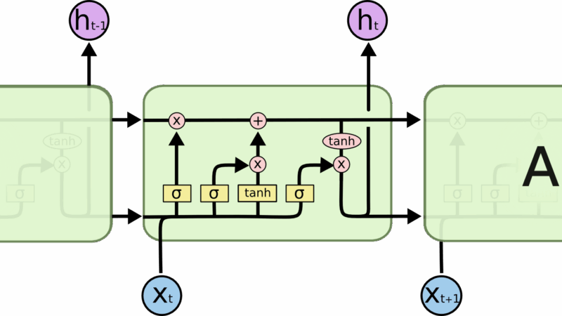
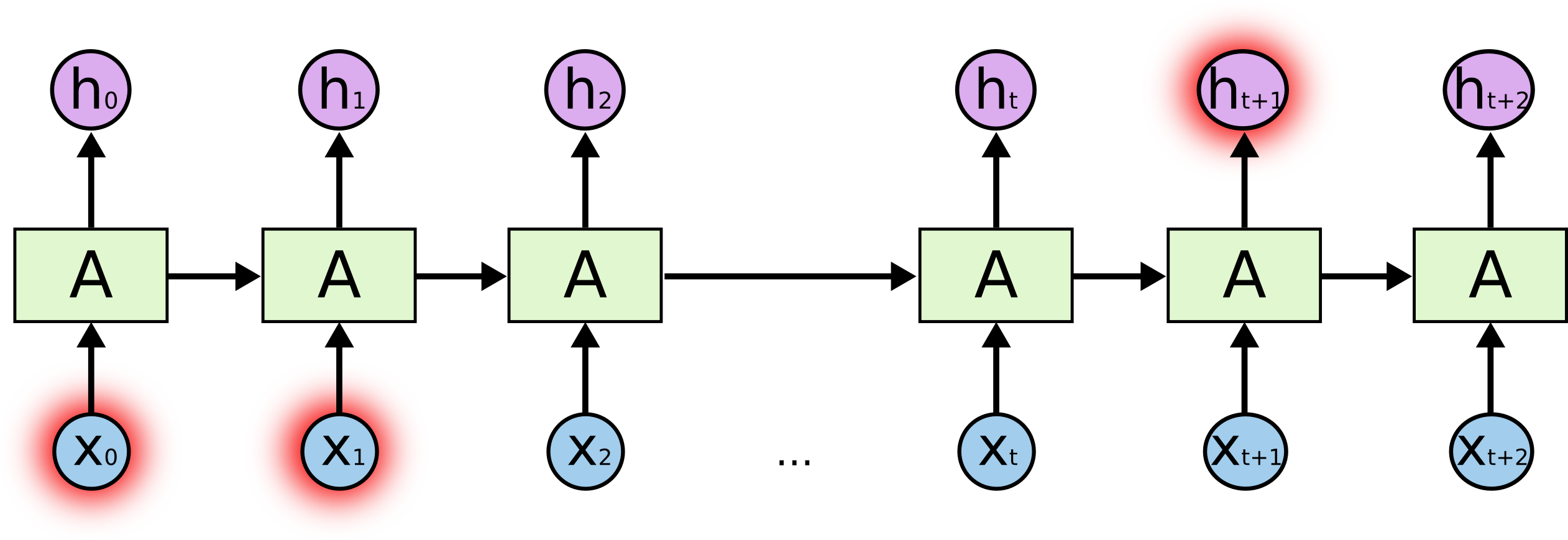
Sentiment Analysis with RNN End to End Project: A Technical Exploration
In today’s digital landscape, understanding sentiment from text data has become a crucial component for businesses and researchers alike. This blog post explores an end-to-end implementation of a sentiment analysis system using Recurrent Neural Networks (RNNs), with a detailed examination of the underlying code, architecture decisions, and deployment strategy.
Try the Sentiment WebApp: model Accuracy > 90%
IMDB Sentiment Analysis Webapp
Analyze the sentiment of any IMDB review using our Sentiment Analysis Tool
The Sentiment Analysis RNN project by Tejas K provides a comprehensive implementation of sentiment analysis that takes raw text as input and classifies it into positive, negative, or neutral categories. What makes this project stand out is its careful attention to the entire machine learning pipeline from data preprocessing to deployment.
Let’s delve into the technical aspects of this implementation.
Data Preprocessing: The Foundation
The quality of any NLP model heavily depends on how well the text data is preprocessed. The project implements several crucial preprocessing steps:
def preprocess_text(text):
    # Convert to lowercase
    text = text.lower()

    # Remove HTML tags
    text = re.sub(r'<.*?>', '', text)

    # Remove special characters and numbers
    text = re.sub(r'[^a-zA-Z\s]', '', text)

    # Tokenize
    tokens = word_tokenize(text)

    # Remove stopwords
    stop_words = set(stopwords.words('english'))
    tokens = [word for word in tokens if word not in stop_words]

    # Lemmatization
    lemmatizer = WordNetLemmatizer()
    tokens = [lemmatizer.lemmatize(word) for word in tokens]

    return ' '.join(tokens)
This preprocessing function performs several important operations:
Converting text to lowercase to ensure consistent processing
Removing HTML tags that might be present in web-scraped data
Filtering out special characters and numbers to focus on alphabetic content
Tokenizing the text into individual words
Removing stopwords (common words like “the”, “and”, etc.) that typically don’t carry sentiment
Lemmatizing words to reduce them to their base form
Building the Vocabulary: Tokenization and Embedding
Before feeding text to an RNN, we need to convert words into numerical vectors. The project implements a vocabulary builder and embedding mechanism:
class Vocabulary:
    def __init__(self, max_size=None):
        self.word2idx = {"<PAD>": 0, "<UNK>": 1}
        self.idx2word = {0: "<PAD>", 1: "<UNK>"}
        self.word_count = {}
        self.max_size = max_size

    def add_word(self, word):
        if word not in self.word_count:
            self.word_count[word] = 1
        else:
            self.word_count[word] += 1

    def build_vocab(self):
        # Sort words by frequency
        sorted_words = sorted(self.word_count.items(), key=lambda x: x[1], reverse=True)

        # Take only max_size most common words if specified
        if self.max_size:
            sorted_words = sorted_words[:self.max_size-2]  # -2 for <PAD> and <UNK>

        # Add words to dictionaries
        for word, _ in sorted_words:
            idx = len(self.word2idx)
            self.word2idx[word] = idx
            self.idx2word[idx] = word

    def text_to_indices(self, text, max_length=None):
        words = text.split()
        indices = [self.word2idx.get(word, self.word2idx["<UNK>"]) for word in words]

        if max_length:
            if len(indices) > max_length:
                indices = indices[:max_length]
            else:
                indices += [self.word2idx["<PAD>"]] * (max_length - len(indices))

        return indices
This vocabulary class:
Maintains mappings between words and their numerical indices
Counts word frequencies to build a vocabulary of the most common words
Handles unknown words with a special <UNK> token
Pads sequences to a consistent length with a <PAD> token
Converts text to sequences of indices for model processing
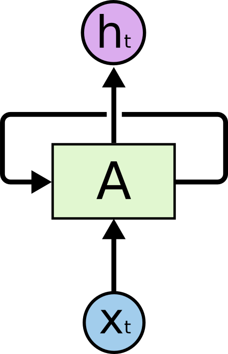
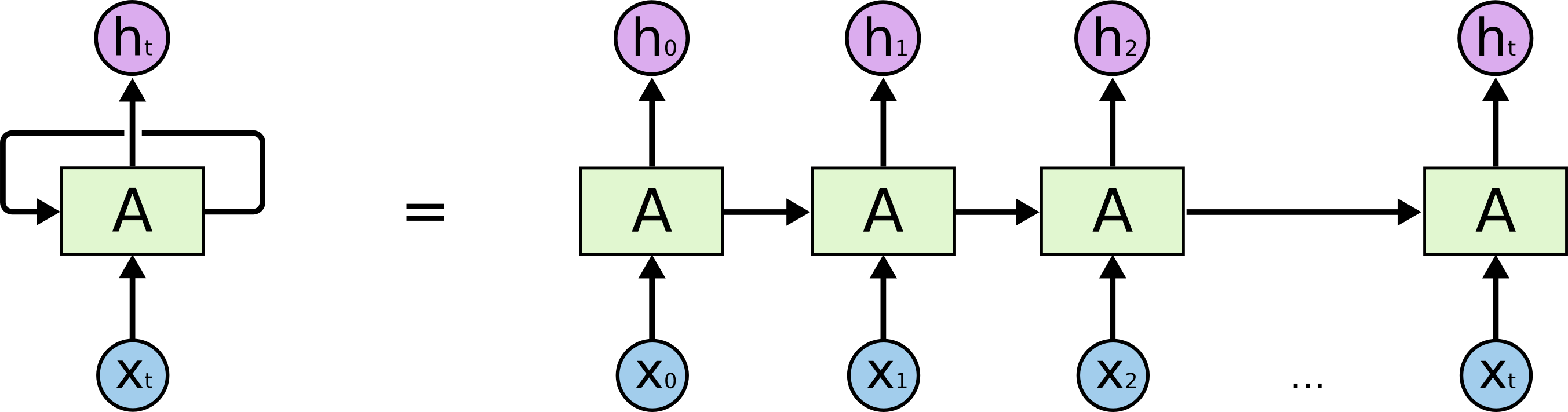
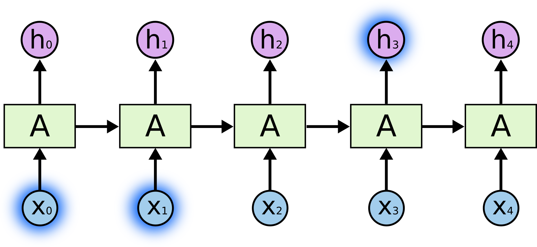
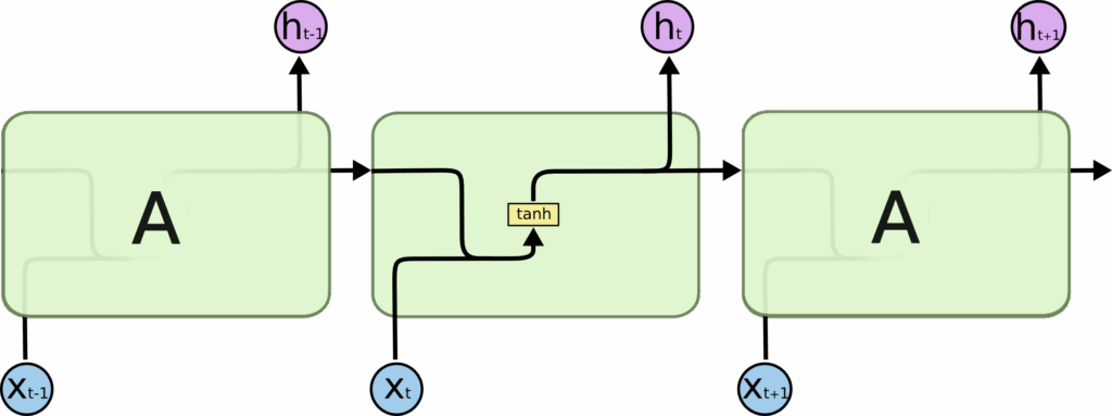
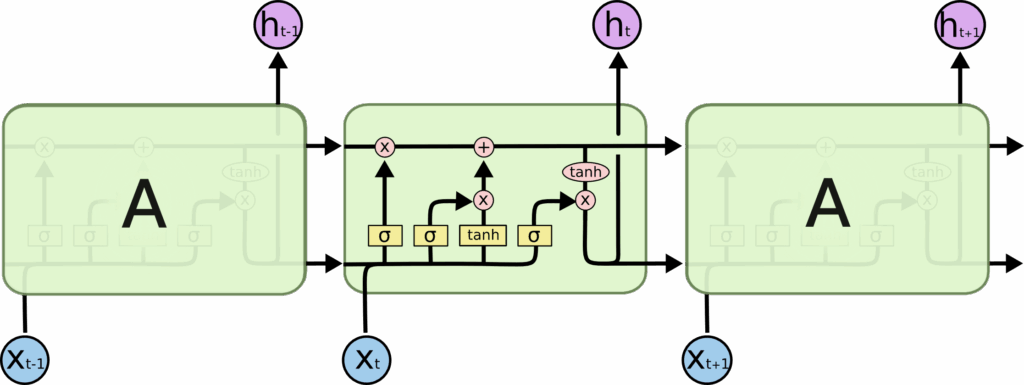
The Core: RNN Model Architecture
The heart of the project is the RNN model architecture. The implementation uses PyTorch to build a flexible model that can be configured with different RNN cell types (LSTM or GRU) and embedding dimensions:
class SentimentRNN(nn.Module):
    def __init__(self, vocab_size, embedding_dim, hidden_dim, output_dim, n_layers,
                 bidirectional, dropout, pad_idx, cell_type='lstm'):
        super().__init__()

        self.embedding = nn.Embedding(vocab_size, embedding_dim, padding_idx=pad_idx)

        if cell_type.lower() == 'lstm':
            self.rnn = nn.LSTM(embedding_dim,
                              hidden_dim,
                              num_layers=n_layers,
                              bidirectional=bidirectional,
                              dropout=dropout if n_layers > 1 else 0,
                              batch_first=True)
        elif cell_type.lower() == 'gru':
            self.rnn = nn.GRU(embedding_dim,
                             hidden_dim,
                             num_layers=n_layers,
                             bidirectional=bidirectional,
                             dropout=dropout if n_layers > 1 else 0,
                             batch_first=True)
        else:
            raise ValueError("cell_type must be 'lstm' or 'gru'")

        self.fc = nn.Linear(hidden_dim * 2 if bidirectional else hidden_dim, output_dim)
        self.dropout = nn.Dropout(dropout)

    def forward(self, text, text_lengths):
        # text = [batch size, seq length]
        embedded = self.dropout(self.embedding(text))
        # embedded = [batch size, seq length, embedding dim]

        # Pack sequence for RNN efficiency
        packed_embedded = nn.utils.rnn.pack_padded_sequence(embedded, text_lengths.cpu(),
                                                         batch_first=True, enforce_sorted=False)

        if isinstance(self.rnn, nn.LSTM):
            packed_output, (hidden, _) = self.rnn(packed_embedded)
        else:  # GRU
            packed_output, hidden = self.rnn(packed_embedded)

        # hidden = [n layers * n directions, batch size, hidden dim]

        # If bidirectional, concatenate the final forward and backward hidden states
        if self.rnn.bidirectional:
            hidden = self.dropout(torch.cat((hidden[-2,:,:], hidden[-1,:,:]), dim=1))
        else:
            hidden = self.dropout(hidden[-1,:,:])

        # hidden = [batch size, hidden dim * n directions]

        return self.fc(hidden)
This model includes several key components:
An embedding layer that converts word indices to dense vectors
A configurable RNN layer (either LSTM or GRU) that processes the sequence
Support for bidirectional processing to capture context from both directions
Dropout for regularization to prevent overfitting
A final fully connected layer for classification
Efficient sequence packing to handle variable-length inputs
Training the Model: The Learning Process
The training loop implements several best practices for deep learning:
Setting the model to evaluation mode with model.eval()
Using torch.no_grad() to disable gradient calculation for efficiency
Not performing backward passes or optimizer steps
Model Deployment: From PyTorch to Streamlit
The project’s deployment strategy involves exporting the trained PyTorch model to TorchScript for production use:
def export_model(model, vocab):
    model.eval()

    # Create a script module from the PyTorch model
    example_text = torch.randint(0, len(vocab), (1, 10))
    example_lengths = torch.tensor([10])

    traced_model = torch.jit.trace(model, (example_text, example_lengths))

    # Save the scripted model
    torch.jit.save(traced_model, "sentiment_model.pt")

    # Save the vocabulary
    with open("vocab.json", "w") as f:
        json.dump({
            "word2idx": vocab.word2idx,
            "idx2word": {int(k): v for k, v in vocab.idx2word.items()}
        }, f)
The exported model is then integrated into a Streamlit application for easy access:
def load_model():
    # Load the TorchScript model
    model = torch.jit.load("sentiment_model.pt")

    # Load vocabulary
    with open("vocab.json", "r") as f:
        vocab_data = json.load(f)

    # Recreate vocabulary object
    vocab = Vocabulary()
    vocab.word2idx = vocab_data["word2idx"]
    vocab.idx2word = {int(k): v for k, v in vocab_data["idx2word"].items()}

    return model, vocab

def predict_sentiment(model, vocab, text):
    # Preprocess text
    processed_text = preprocess_text(text)

    # Convert to indices
    indices = vocab.text_to_indices(processed_text, max_length=100)
    tensor = torch.LongTensor(indices).unsqueeze(0)  # Add batch dimension
    length = torch.tensor([len(indices)])

    # Make prediction
    model.eval()
    with torch.no_grad():
        prediction = model(tensor, length)

    # Get probability using softmax
    probabilities = F.softmax(prediction, dim=1)

    # Get predicted class
    predicted_class = torch.argmax(prediction, dim=1).item()

    # Map to sentiment
    sentiment_map = {0: "Negative", 1: "Neutral", 2: "Positive"}

    return {
        "sentiment": sentiment_map[predicted_class],
        "confidence": probabilities[0][predicted_class].item(),
        "probabilities": {
            sentiment_map[i]: prob.item() for i, prob in enumerate(probabilities[0])
        }
    }
The Streamlit application code brings everything together in a user-friendly interface:
def main():
    st.title("Sentiment Analysis with RNN")

    model, vocab = load_model()

    st.write("Enter text to analyze its sentiment:")
    user_input = st.text_area("Text input", "")

    if st.button("Analyze Sentiment"):
        if user_input:
            with st.spinner("Analyzing..."):
                result = predict_sentiment(model, vocab, user_input)

            st.write(f"**Sentiment:** {result['sentiment']}")
            st.write(f"**Confidence:** {result['confidence']*100:.2f}%")

            # Display probabilities
            st.write("### Probability Distribution")
            for sentiment, prob in result['probabilities'].items():
                st.write(f"{sentiment}: {prob*100:.2f}%")
                st.progress(prob)
        else:
            st.warning("Please enter some text to analyze.")

if __name__ == "__main__":
    main()
The iframe parameters and styling ensure:
The dark theme specified with embed_options=dark_theme
Responsive design that works on different screen sizes
Clean integration with the WordPress site’s aesthetics
Proper sizing to accommodate the application’s interface
Performance Optimization and Model Improvements
The project implements several performance optimizations:
Batch processing during training to improve GPU utilization:
def train_with_early_stopping(model, train_iterator, valid_iterator,
                             optimizer, criterion, patience=5):
    best_valid_loss = float('inf')
    epochs_without_improvement = 0

    for epoch in range(max_epochs):
        train_loss, train_acc = train_model(model, train_iterator, optimizer, criterion)
        valid_loss, valid_acc = evaluate_model(model, valid_iterator, criterion)

        if valid_loss < best_valid_loss:
            best_valid_loss = valid_loss
            torch.save(model.state_dict(), 'best-model.pt')
            epochs_without_improvement = 0
        else:
            epochs_without_improvement += 1

        print(f'Epoch: {epoch+1}')
        print(f'\tTrain Loss: {train_loss:.3f} | Train Acc: {train_acc*100:.2f}%')
        print(f'\tVal. Loss: {valid_loss:.3f} | Val. Acc: {valid_acc*100:.2f}%')

        if epochs_without_improvement >= patience:
            print(f'Early stopping after {epoch+1} epochs')
            break

    # Load the best model
    model.load_state_dict(torch.load('best-model.pt'))
    return model
Learning rate scheduling for better convergence:
optimizer = optim.Adam(model.parameters(), lr=2e-4)
scheduler = optim.lr_scheduler.ReduceLROnPlateau(optimizer, mode='min',
                                                factor=0.5, patience=2)

# In training loop
scheduler.step(valid_loss)
Conclusion: Putting It All Together
The Sentiment Analysis RNN project demonstrates how to build a complete NLP system from data preprocessing to web deployment. Key technical takeaways include:
Effective text preprocessing is crucial for good model performance
RNNs (particularly LSTMs and GRUs) excel at capturing sequential dependencies in text
Proper training techniques like early stopping and learning rate scheduling improve model quality
Model export and deployment bridges the gap between development and production
Web integration makes the model accessible to end-users without technical knowledge
By embedding the Streamlit application in a WordPress site, this technical solution becomes accessible to a wider audience, showcasing how advanced NLP techniques can be applied to practical problems.
The combination of robust model architecture, efficient training procedures, and user-friendly deployment makes this project an excellent case study in applied deep learning for natural language processing.
You can explore the full implementation on GitHub or try the live demo at Streamlit App.
By Tejas Kamble – AI/ML Developer & Researcher | tejaskamble.com
Introduction
Have you ever used the Netflix search bar and instantly seen suggestions that seem to know exactly what you’re looking for—even before you finish typing? Inspired by this, I created a Netflix Search Engine using NLP Text Suggestions — a project that bridges the power of natural language processing (NLP) with real-time search functionalities.
In this post, I’ll walk you through the codebase hosted on my GitHub: Netflix_Search_Engine_NLP_Text_suggestion, breaking down each important part, from data loading and text preprocessing to building the suggestion logic and deploying it using Flask.
TF-IDF is powerful for information retrieval tasks.
Even a simple cosine similarity search can replicate sophisticated autocomplete behavior.
Flask makes it easy to bring machine learning to the web.
What’s Next?
Here are a few ways I plan to extend this project:
Use BERT or Sentence Transformers for semantic similarity.
Add spell correction and synonym support.
Deploy it on Render, Heroku, or HuggingFace Spaces.
Add a recommendation engine using genres, cast similarity, or collaborative filtering.
🧑💻 About Me
I’m Tejas Kamble, an AI/ML Developer & Researcher passionate about building intelligent, ethical, and multilingual human-computer interaction systems. I focus on:
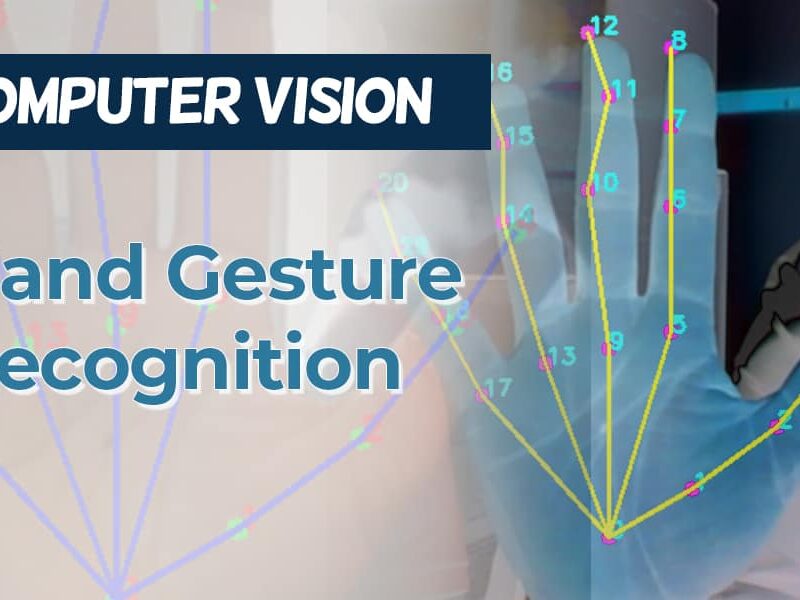
In today’s digital era, the way we interact with computers continues to evolve. Beyond the traditional keyboard and mouse, gesture recognition represents one of the most intuitive forms of human-computer interaction. By leveraging computer vision techniques and machine learning, we can create systems that interpret hand movements and translate them into computer commands.
This blog explores the development of a gesture-controlled mouse system that allows users to control their cursor and perform clicks using only hand movements captured by a webcam. We’ll dive deep into the underlying computer vision technologies, implementation details, and practical considerations for building such a system.
The Science Behind Gesture Recognition
Computer Vision Fundamentals
Computer vision is the field that enables computers to derive meaningful information from digital images or videos. At its core, it involves:
Image Acquisition: Capturing visual data through cameras or sensors
Image Processing: Manipulating images to enhance features or reduce noise
Feature Detection: Identifying points of interest within an image
Pattern Recognition: Classifying patterns or objects within the visual data
For gesture control systems, we need reliable methods to detect hands, identify their landmarks (key points), and interpret their movements.
Hand Detection and Tracking
Modern hand tracking systems typically follow a two-stage approach:
Hand Detection: Locating the hand within the frame
Landmark Detection: Identifying specific points on the hand (fingertips, joints, palm center)
Historically, approaches included:
Color-based segmentation: Isolating hand regions based on skin color
Background subtraction: Identifying moving objects against a static background
Feature-based methods: Using handcrafted features like Haar cascades or HOG
Today’s state-of-the-art systems leverage deep learning, specifically convolutional neural networks (CNNs), for both detection and landmark identification.
MediaPipe Hands
Google’s MediaPipe Hands is currently one of the most accessible and accurate hand tracking solutions available. It provides:
Real-time hand detection
21 3D landmarks per hand
Support for multiple hands
Cross-platform compatibility
MediaPipe uses a pipeline approach:
A palm detector that locates hand regions
A hand landmark model that identifies 21 key points
A gesture recognition system built on these landmarks
Each landmark corresponds to a specific anatomical feature of the hand:
Wrist point
Thumb (4 points)
Index finger (4 points)
Middle finger (4 points)
Ring finger (4 points)
Pinky finger (4 points)
Sample Code
import cvzone
import cv2

cap = cv2.VideoCapture(0)
cap.set(3, 1280)
cap.set(4, 720)
detector = cvzone.HandDetector(detectionCon=0.5, maxHands=1)

while True:
    # Get image frame
    success, img = cap.read()

    # Find the hand and its landmarks
    img = detector.findHands(img)
    lmList, bbox = detector.findPosition(img)

    # Display
    cv2.imshow("Image", img)
    cv2.waitKey(1)
Building a Gesture-Controlled Mouse
System Architecture
Our gesture mouse system consists of several interconnected components:
Input Processing: Captures and processes webcam input
Hand Detection: Identifies hands in the frame
Landmark Extraction: Locates the 21 key points on each hand
Gesture Recognition: Interprets specific hand configurations as commands
Command Execution: Translates gestures into mouse actions
Required Technologies and Libraries
To implement this system, we’ll use:
OpenCV: For webcam capture and image processing
MediaPipe: For hand detection and landmark tracking
PyAutoGUI: For programmatically controlling the mouse
NumPy: For efficient numerical operations
Implementation Details
Let’s explore the core functionality of our gesture-controlled mouse system:
1. Setting Up the Environment
First, we initialize the necessary libraries and configure MediaPipe for hand tracking:
import cv2
import mediapipe as mp
import pyautogui
import numpy as np
import time

# Initialize MediaPipe Hand solution
mp_hands = mp.solutions.hands
hands = mp_hands.Hands(
    static_image_mode=False,
    max_num_hands=1,
    min_detection_confidence=0.7,
    min_tracking_confidence=0.5
)
mp_drawing = mp.solutions.drawing_utils

# Get screen dimensions for mapping hand position to screen coordinates
screen_width, screen_height = pyautogui.size()
The MediaPipe configuration includes several important parameters:
static_image_mode=False: Optimizes for video sequence tracking
max_num_hands=1: Limits detection to one hand for simplicity
min_detection_confidence=0.7: Sets the threshold for hand detection
min_tracking_confidence=0.5: Sets the threshold for tracking continuation
2. Capturing and Processing Video
Next, we set up the webcam capture and create the main processing loop:
# Get webcam
cap = cv2.VideoCapture(0)

while cap.isOpened():
    success, image = cap.read()
    if not success:
        print("Failed to capture image from webcam.")
        continue

    # Flip the image horizontally for a more intuitive mirror view
    image = cv2.flip(image, 1)

    # Convert BGR image to RGB for MediaPipe
    rgb_image = cv2.cvtColor(image, cv2.COLOR_BGR2RGB)

    # Process the image and detect hands
    results = hands.process(rgb_image)
The horizontal flip creates a mirror-like experience, making the interaction more intuitive for users.
3. Hand Landmark Detection
Once we have processed the image, we extract and visualize the hand landmarks:
# Draw hand landmarks if detected
if results.multi_hand_landmarks:
    for hand_landmarks in results.multi_hand_landmarks:
        mp_drawing.draw_landmarks(
            image, hand_landmarks, mp_hands.HAND_CONNECTIONS)

        # Get the landmarks as a list
        landmarks = hand_landmarks.landmark

        # Process landmarks for mouse control...
Each detected hand provides 21 landmarks with normalized coordinates:
x, y: Normalized to [0.0, 1.0] within the image
z: Represents depth with the wrist as origin (negative values are toward the camera)
4. Implementing Mouse Movement
To control mouse movement, we map hand position to screen coordinates:
# Smoothing factors
smoothing = 5
prev_x, prev_y = 0, 0

# Inside the main loop:
# Using wrist position for mouse control
wrist = landmarks[mp_hands.HandLandmark.WRIST]
x = int(wrist.x * screen_width)
y = int(wrist.y * screen_height)

# Apply smoothing for more stable cursor movement
prev_x = prev_x + (x - prev_x) / smoothing
prev_y = prev_y + (y - prev_y) / smoothing

# Move the mouse
pyautogui.moveTo(prev_x, prev_y)
The smoothing factor reduces jitter by creating a weighted average between the current and previous positions, resulting in more fluid cursor movement.
5. Gesture Recognition for Mouse Clicks
For click actions, we detect finger tap gestures:
def detect_finger_tap(landmarks, finger_tip_idx, finger_pip_idx):
    """Detect if a finger is tapped (tip close to palm)"""
    tip = landmarks[finger_tip_idx]
    pip = landmarks[finger_pip_idx]

    # Calculate vertical distance between tip and pip
    distance = abs(tip.y - pip.y)

    # If tip is below pip and close enough, it's a tap
    return tip.y > pip.y and distance < tap_threshold

# In the main loop:
# Detect index finger tap for left click
if detect_finger_tap(landmarks, mp_hands.HandLandmark.INDEX_FINGER_TIP, mp_hands.HandLandmark.INDEX_FINGER_PIP):
    current_time = time.time()
    if current_time - last_index_tap_time > tap_cooldown:
        print("Left click")
        pyautogui.click()
        last_index_tap_time = current_time

# Detect middle finger tap for right click
if detect_finger_tap(landmarks, mp_hands.HandLandmark.MIDDLE_FINGER_TIP, mp_hands.HandLandmark.MIDDLE_FINGER_PIP):
    current_time = time.time()
    if current_time - last_middle_tap_time > tap_cooldown:
        print("Right click")
        pyautogui.rightClick()
        last_middle_tap_time = current_time
The tap detection works by:
Measuring the vertical distance between a fingertip and its corresponding PIP joint
Identifying a tap when the fingertip moves below the joint and within a certain distance threshold
Implementing a cooldown period to prevent accidental multiple clicks
Implementing Scrolling Functionality
Scrolling is an essential feature for navigating documents and webpages. Let’s implement smooth scrolling control using hand gestures.
1. Pinch-to-Scroll Implementation
One of the most intuitive ways to implement scrolling is through a pinch gesture between the thumb and ring finger, followed by vertical movement:
# Global variables for tracking scroll state
scroll_active = False
scroll_start_y = 0
last_scroll_time = 0
scroll_cooldown = 0.05  # Seconds between scroll actions
scroll_sensitivity = 1.0  # Adjustable scroll sensitivity

def detect_scroll_gesture(landmarks):
    """Detect thumb and ring finger pinch for scrolling"""
    thumb_tip = landmarks[mp_hands.HandLandmark.THUMB_TIP]
    ring_tip = landmarks[mp_hands.HandLandmark.RING_FINGER_TIP]

    # Calculate distance between thumb and ring finger
    distance = np.sqrt((thumb_tip.x - ring_tip.x)**2 + (thumb_tip.y - ring_tip.y)**2)

    # If thumb and ring finger are close enough, it's a pinch
    return distance < 0.07  # Threshold value may need adjustment

# In the main loop:
if results.multi_hand_landmarks:
    landmarks = results.multi_hand_landmarks[0].landmark

    # Check for scroll gesture
    is_scroll_gesture = detect_scroll_gesture(landmarks)

    # Get middle point between thumb and ring finger for tracking
    if is_scroll_gesture:
        thumb_tip = landmarks[mp_hands.HandLandmark.THUMB_TIP]
        ring_tip = landmarks[mp_hands.HandLandmark.RING_FINGER_TIP]
        current_y = (thumb_tip.y + ring_tip.y) / 2

        # Initialize scroll if just started pinching
        if not scroll_active:
            scroll_active = True
            scroll_start_y = current_y
        else:
            # Calculate scroll distance
            current_time = time.time()
            if current_time - last_scroll_time > scroll_cooldown:
                # Convert movement to scroll amount
                scroll_amount = int((current_y - scroll_start_y) * 20 * scroll_sensitivity)

                if abs(scroll_amount) > 0:
                    # Scroll up or down
                    pyautogui.scroll(-scroll_amount)  # Negative because screen coordinates are inverted
                    scroll_start_y = current_y  # Reset start position
                    last_scroll_time = current_time
    else:
        scroll_active = False
This implementation:
Detects a pinch between the thumb and ring finger
Tracks the vertical movement of the pinch
Converts the movement to scrolling actions
Uses a cooldown mechanism to prevent too many scroll events
Applies sensitivity settings to adjust scroll speed
2. Alternative: Two-Finger Scroll Gesture
For users who might find the pinch gesture challenging, we can implement an alternative two-finger scroll method:
def detect_two_finger_scroll(landmarks):
    """Detect index and middle finger extended for scrolling"""
    index_tip = landmarks[mp_hands.HandLandmark.INDEX_FINGER_TIP]
    index_pip = landmarks[mp_hands.HandLandmark.INDEX_FINGER_PIP]
    middle_tip = landmarks[mp_hands.HandLandmark.MIDDLE_FINGER_TIP]
    middle_pip = landmarks[mp_hands.HandLandmark.MIDDLE_FINGER_PIP]

    # Check if both fingers are extended (tips above pips)
    index_extended = index_tip.y < index_pip.y
    middle_extended = middle_tip.y < middle_pip.y

    # Check if other fingers are curled
    ring_tip = landmarks[mp_hands.HandLandmark.RING_FINGER_TIP]
    ring_pip = landmarks[mp_hands.HandLandmark.RING_FINGER_PIP]
    pinky_tip = landmarks[mp_hands.HandLandmark.PINKY_TIP]
    pinky_pip = landmarks[mp_hands.HandLandmark.PINKY_PIP]

    ring_curled = ring_tip.y > ring_pip.y
    pinky_curled = pinky_tip.y > pinky_pip.y

    # Return true if index and middle extended, others curled
    return index_extended and middle_extended and ring_curled and pinky_curled
This can then be integrated into the main loop similarly to the pinch gesture method.
3. Visual Feedback for Scrolling
Providing visual feedback helps users understand when the system recognizes their scroll gesture:
# Inside the main loop, when scroll gesture is detected:
if is_scroll_gesture:
    # Draw a visual indicator for active scrolling
    cv2.circle(image, (50, 50), 20, (0, 255, 0), -1)  # Green circle when scrolling
    cv2.putText(image, f"Scrolling {'UP' if scroll_amount < 0 else 'DOWN'}",
                (75, 50), cv2.FONT_HERSHEY_SIMPLEX, 0.7, (0, 255, 0), 2)
Adjustable Mouse Sensitivity
Different users have different preferences for cursor speed and precision. Let’s implement adjustable sensitivity controls:
1. Adding Sensitivity Settings
First, we’ll define sensitivity parameters that can be adjusted:
We need to modify our mouse movement logic to incorporate the sensitivity setting:
# Inside the main loop, when calculating cursor position:
wrist = landmarks[mp_hands.HandLandmark.WRIST]

# Get raw coordinates
raw_x = wrist.x * screen_width
raw_y = wrist.y * screen_height

# Calculate center of screen
center_x = screen_width / 2
center_y = screen_height / 2

# Apply sensitivity to the distance from center
offset_x = (raw_x - center_x) * mouse_sensitivity
offset_y = (raw_y - center_y) * mouse_sensitivity

# Calculate final position
x = int(center_x + offset_x)
y = int(center_y + offset_y)

# Apply smoothing for stable cursor movement
prev_x = prev_x + (x - prev_x) / smoothing
prev_y = prev_y + (y - prev_y) / smoothing

# Move the mouse
pyautogui.moveTo(prev_x, prev_y)
This approach:
Calculates the cursor position relative to the center of the screen
Applies the sensitivity factor to the offset from center
Ensures that low sensitivity gives fine control, while high sensitivity allows rapid movement across the screen
3. Gesture-Based Sensitivity Adjustment
Now we’ll implement gestures to adjust sensitivity on-the-fly:
# Global variables for tracking the last sensitivity adjustment
last_sensitivity_change_time = 0
sensitivity_change_cooldown = 1.0  # Seconds between adjustments

def detect_increase_sensitivity_gesture(landmarks):
    """Detect gesture for increasing sensitivity (pinky and thumb pinch)"""
    thumb_tip = landmarks[mp_hands.HandLandmark.THUMB_TIP]
    pinky_tip = landmarks[mp_hands.HandLandmark.PINKY_TIP]

    distance = np.sqrt((thumb_tip.x - pinky_tip.x)**2 + (thumb_tip.y - pinky_tip.y)**2)
    return distance < 0.07

def detect_decrease_sensitivity_gesture(landmarks):
    """Detect gesture for decreasing sensitivity (thumb touching wrist)"""
    thumb_tip = landmarks[mp_hands.HandLandmark.THUMB_TIP]
    wrist = landmarks[mp_hands.HandLandmark.WRIST]

    distance = np.sqrt((thumb_tip.x - wrist.x)**2 + (thumb_tip.y - wrist.y)**2)
    return distance < 0.12

# In the main loop:
# Check for sensitivity adjustment gestures
current_time = time.time()
if current_time - last_sensitivity_change_time > sensitivity_change_cooldown:
    if detect_increase_sensitivity_gesture(landmarks):
        mouse_sensitivity = min(mouse_sensitivity + sensitivity_step, sensitivity_max)
        print(f"Sensitivity increased to: {mouse_sensitivity:.1f}")
        last_sensitivity_change_time = current_time

    elif detect_decrease_sensitivity_gesture(landmarks):
        mouse_sensitivity = max(mouse_sensitivity - sensitivity_step, sensitivity_min)
        print(f"Sensitivity decreased to: {mouse_sensitivity:.1f}")
        last_sensitivity_change_time = current_time
4. On-Screen Sensitivity Display
To help users understand the current sensitivity level, we can display it on the screen:
# Inside the main loop, after handling sensitivity adjustments:
# Display current sensitivity on screen
cv2.putText(image, f"Sensitivity: {mouse_sensitivity:.1f}",
            (10, image.shape[0] - 20), cv2.FONT_HERSHEY_SIMPLEX,
            0.7, (0, 255, 0), 2)
5. UI Controls for Sensitivity Adjustment
For a more user-friendly experience, we can add GUI controls using OpenCV:
# Create a sensitivity slider using OpenCV
def create_control_window():
    cv2.namedWindow('Mouse Controls')
    cv2.createTrackbar('Sensitivity', 'Mouse Controls',
                       int(mouse_sensitivity * 10),
                       int(sensitivity_max * 10),
                       on_sensitivity_change)
    cv2.createTrackbar('Scroll Speed', 'Mouse Controls',
                       int(scroll_sensitivity * 10),
                       int(sensitivity_max * 10),
                       on_scroll_sensitivity_change)

def on_sensitivity_change(value):
    global mouse_sensitivity
    mouse_sensitivity = value / 10.0

def on_scroll_sensitivity_change(value):
    global scroll_sensitivity
    scroll_sensitivity = value / 10.0

# Call at the beginning of your program
create_control_window()
6. Configuration File for Persistent Settings
To remember user preferences between sessions, we can save settings to a configuration file:
import json
import os

config_file = "gesture_mouse_config.json"

def save_settings():
    """Save current settings to a JSON file"""
    settings = {
        "mouse_sensitivity": mouse_sensitivity,
        "scroll_sensitivity": scroll_sensitivity,
        "smoothing": smoothing
    }

    with open(config_file, 'w') as f:
        json.dump(settings, f)

    print("Settings saved!")

def load_settings():
    """Load settings from a JSON file if it exists"""
    global mouse_sensitivity, scroll_sensitivity, smoothing

    if os.path.exists(config_file):
        try:
            with open(config_file, 'r') as f:
                settings = json.load(f)

            mouse_sensitivity = settings.get("mouse_sensitivity", mouse_sensitivity)
            scroll_sensitivity = settings.get("scroll_sensitivity", scroll_sensitivity)
            smoothing = settings.get("smoothing", smoothing)

            print("Settings loaded!")
        except:
            print("Error loading settings. Using defaults.")

# Load settings at startup
load_settings()

# Add keyboard event to save settings:
# (inside the main loop)
key = cv2.waitKey(1) & 0xFF
if key == ord('s'):
    save_settings()
Technical Challenges and Solutions
Challenge 1: Hand Detection Stability
Problem: Hand detection can be inconsistent under varying lighting conditions or when the hand moves quickly.
Solution: Multiple approaches can improve stability:
Adjust MediaPipe confidence thresholds based on your environment
Implement background removal techniques to isolate the hand
Use temporal filtering to reject spurious detections
Challenge 2: Gesture Recognition Accuracy
Problem: Distinguishing intentional gestures from natural hand movements.
Solution:
Define clear gesture thresholds
Implement gesture “holding” requirements (e.g., maintain a gesture for 300ms)
Add visual feedback to help users understand when gestures are recognized
Challenge 3: Cursor Stability
Problem: Direct mapping of hand position to cursor coordinates can result in jittery movement.
Solution:
Implement motion smoothing algorithms (like our weighted average approach)
Use Kalman filtering for more sophisticated motion prediction
Create a “deadzone” where small hand movements don’t affect the cursor
Challenge 4: Fatigue and Ergonomics
Problem: Holding the hand in mid-air causes user fatigue over time.
Solution:
Implement a “clutch” mechanism that enables/disables control
Design gestures that allow for natural hand positions
Consider relative positioning rather than absolute positioning
Challenge 5: Scroll Precision
Problem: Scrolling can be too sensitive or jerky with direct hand movement mapping.
Solution:
Implement non-linear scroll response curves
Add “scroll momentum” for smoother continuous scrolling
Provide visual feedback about scroll speed and direction
# Non-linear scroll response curve
def apply_scroll_curve(movement):
    """Apply a non-linear curve to make small movements more precise"""
    # Square the movement but keep the sign
    sign = 1 if movement >= 0 else -1
    magnitude = abs(movement)

    # Apply curve: square for values > 0.1, linear for smaller values
    if magnitude > 0.1:
        result = sign * ((magnitude - 0.1) ** 2) * 2 + (sign * 0.1)
    else:
        result = sign * magnitude

    return result
Advanced Features and Improvements
Enhancing Mouse Movement
For more precise control, we can improve the mapping between hand position and cursor movement:
# Define a region of interest in the camera's field of view
roi_left = 0.2
roi_right = 0.8
roi_top = 0.2
roi_bottom = 0.8

# Map the hand position within this region to screen coordinates
def map_to_screen(x, y):
    screen_x = screen_width * (x - roi_left) / (roi_right - roi_left)
    screen_y = screen_height * (y - roi_top) / (roi_bottom - roi_top)
    return max(0, min(screen_width, screen_x)), max(0, min(screen_height, screen_y))
This approach creates a smaller “active area” within the camera’s view, allowing for more precise movements.
Implementing Additional Gestures
Beyond basic clicking, we can add more complex interactions:
# Track index finger extension status
index_extended = landmarks[mp_hands.HandLandmark.INDEX_FINGER_TIP].y < landmarks[mp_hands.HandLandmark.INDEX_FINGER_PIP].y

# If status changes from extended to not extended while moving, start drag
if prev_index_extended and not index_extended:
    pyautogui.mouseDown()
elif not prev_index_extended and index_extended:
    pyautogui.mouseUp()
Gesture-based shortcuts:
# Detect specific finger configurations
if all_fingers_extended(landmarks):
    # Perform action, like opening task manager
    pyautogui.hotkey('ctrl', 'shift', 'esc')
Calibration System
A calibration system improves accuracy across different users and environments:
def calibrate():
    calibration_points = [(0.1, 0.1), (0.9, 0.1), (0.9, 0.9), (0.1, 0.9)]
    user_points = []

    for point in calibration_points:
        # Prompt user to place hand at this position
        # Record actual hand position
        user_points.append((wrist.x, wrist.y))

    # Create transformation matrix
    transformation = calculate_transformation(calibration_points, user_points)
    return transformation
Performance Optimization
To ensure smooth operation, several optimizations are critical:
1. Frame Rate Management
Processing every frame can be computationally expensive. We can reduce the processing load:
# Process only every n frames
if frame_count % process_every_n_frames == 0:
    # Process hand detection and tracking
else:
    # Use the previous result
2. Resolution Scaling
Lower resolution processing can significantly improve performance:
# Scale down the image for processing
process_scale = 0.5
small_frame = cv2.resize(image, (0, 0), fx=process_scale, fy=process_scale)

# Process the smaller image
results = hands.process(small_frame)

# Scale coordinates back up when using them
x = int(landmark.x / process_scale)
y = int(landmark.y / process_scale)
3. Multi-threading
Separating video capture from processing improves responsiveness:
def capture_thread():
    while running:
        ret, frame = cap.read()
        if ret:
            frame_queue.put(frame)

def process_thread():
    while running:
        if not frame_queue.empty():
            frame = frame_queue.get()
            # Process the frame
Real-World Applications
Gesture control systems have numerous practical applications beyond cursor control:
Accessibility: Enables computer use for people with mobility impairments
Medical Environments: Allows for touchless interaction in sterile settings
Presentations: Facilitates natural interaction with slides and content
Gaming: Creates immersive control experiences without specialized hardware
Smart Home Control: Enables intuitive interaction with IoT devices
Virtual Reality: Provides hand tracking for more realistic VR experiences
Challenges and Future Directions
While powerful, gesture control systems face several ongoing challenges:
Technical Limitations
Occlusion: Fingers may be hidden from the camera’s view
Background Complexity: Busy environments can confuse hand detection
Lighting Sensitivity: Performance varies with lighting conditions
Camera Limitations: Low frame rates or resolution affect tracking quality
Future Research Directions
Multi-modal Integration: Combining gestures with voice commands or eye tracking
Context-aware Gestures: Adapting to different applications automatically
Transfer Learning: Applying knowledge from one gesture domain to another
Edge Processing: Moving computations to specialized hardware for better performance
Conclusion
Computer vision-based gesture control represents a significant step forward in human-computer interaction, offering a more natural and intuitive way to control computers. By leveraging libraries like MediaPipe and OpenCV, developers can now create sophisticated gesture recognition systems with relatively modest technical requirements.
Our gesture-controlled mouse system demonstrates the core principles of this technology, with additional features like scrolling and adjustable sensitivity making it truly practical for everyday use. The accessibility and customizability of such systems highlight the exciting possibilities at the intersection of computer vision, machine learning, and human-computer interaction.
Whether for accessibility, specialized environments, or simply for the joy of a more natural interaction, gesture control systems are poised to become an increasingly common part of our digital interfaces.
Code Repository
The complete implementation of the gesture-controlled mouse system described in this blog is available on GitHub at {https://github.com/tejask0512/Hand_Gesture_Mouse_Computer_Vision} . The code is extensively commented to help you understand each component and customize it for your specific needs.
In an era where environmental concerns increasingly shape public policy and personal health decisions, access to real-time air quality data has never been more crucial. The AQI Google Maps project represents an innovative approach to environmental monitoring, combining Google Maps’ familiar interface with critical air quality metrics. This open-source initiative transforms complex environmental data into an accessible visualization tool that can benefit researchers, policymakers, and everyday citizens concerned about the air they breathe.
What is the AQI Google Maps Project?
The AQI (Air Quality Index) Google Maps project is an open-source web application that integrates air quality data with Google Maps to provide a visual representation of air pollution levels across different locations. Developed by Tejas K (GitHub: tejask0512), this project leverages modern web technologies and public APIs to create an interactive map where users can view air quality conditions with intuitive color-coded markers.
Technical Architecture
The project employs a straightforward yet effective technical stack:
Frontend: HTML, CSS, JavaScript
APIs: Google Maps API for mapping functionality, Air Quality APIs for pollution data
Data Visualization: Custom markers and color-coding system
The core functionality revolves around fetching air quality data based on geographic coordinates and rendering this information as color-coded markers on the Google Maps interface. The colors transition from green (good air quality) through yellow and orange to red and purple (hazardous air quality), providing an immediate visual understanding of conditions in different areas.
Deep Dive into AQI Analysis
Understanding the Air Quality Index
The Air Quality Index is a standardized indicator developed by environmental agencies to communicate how polluted the air is and what associated health effects might be. The AQI Google Maps project implements this complex calculation system and presents it in an accessible format.
The AQI typically accounts for multiple pollutants:
Created by chemical reactions between NOx and VOCs
Lung damage, respiratory issues
NO2 (Nitrogen Dioxide)
Vehicles, power plants
Respiratory inflammation
SO2 (Sulfur Dioxide)
Fossil fuel combustion, industrial processes
Respiratory issues, contributes to acid rain
CO (Carbon Monoxide)
Incomplete combustion
Reduces oxygen delivery in bloodstream
The project likely calculates an overall AQI based on the highest concentration of any single pollutant, following the EPA’s approach where:
0-50 (Green): Good air quality with minimal health concerns
51-100 (Yellow): Moderate air quality; unusually sensitive individuals may experience issues
101-150 (Orange): Unhealthy for sensitive groups
151-200 (Red): Unhealthy for all groups
201-300 (Purple): Very unhealthy; may trigger health alerts
301+ (Maroon): Hazardous; serious health effects for entire population
The technical implementation likely includes conversion formulas to normalize different pollutant measurements to the same 0-500 AQI scale.
Real-time Data Processing
A key technical achievement of the project is its ability to process real-time air quality data. This involves:
API Integration: Connecting to air quality data providers through RESTful APIs
Data Parsing: Extracting relevant metrics from JSON/XML responses
Coordinate Mapping: Associating pollution data with precise geographic coordinates
Temporal Synchronization: Managing data freshness and update frequencies
The project handles these operations seamlessly in the background, presenting users with up-to-date information without exposing the complexity of the underlying data acquisition process.
Report Generation Capabilities
One of the project’s valuable features is its ability to generate comprehensive air quality reports. These reports serve multiple purposes:
Types of Reports Generated
Location-specific Snapshots: Detailed breakdowns of current air quality at selected points
Comparative Analysis: Contrasting air quality across multiple locations
Temporal Reports: Tracking air quality changes over time (hourly, daily, weekly)
Pollutant-specific Reports: Focusing on individual contaminants like PM2.5 or O3
Report Components
The reporting system likely includes:
Statistical Summaries: Min/max/mean values for AQI metrics
Health Impact Assessments: Explanations of potential health effects based on current readings
Visualizations: Charts and graphs depicting pollution trends
Contextual Information: Weather conditions that may influence readings
Actionable Recommendations: Suggested activities based on air quality levels
Technical Implementation of Reporting
From a development perspective, the reporting functionality demonstrates sophisticated data processing:
This functionality transforms raw data into actionable intelligence, making the project valuable beyond simple visualization.
AQI and Location Coordinate Data for Machine Learning
Perhaps the most forward-looking aspect of the project is its potential for generating valuable datasets for machine learning applications. The combination of precise geolocation data with corresponding air quality metrics creates numerous possibilities for advanced environmental analysis.
Data Generation for ML Models
The project effectively creates a continuous stream of structured data points with these key attributes:
Geographic Coordinates: Latitude and longitude
Temporal Information: Timestamps for each measurement
Multiple Pollutant Metrics: PM2.5, PM10, O3, NO2, SO2, CO values
Calculated AQI: Overall air quality index
Contextual Metadata: Potentially including weather conditions, urban density, etc.
This multi-dimensional dataset serves as excellent training data for various machine learning models.
Potential ML Applications
With sufficient data collection over time, the following machine learning approaches become possible:
1. Predictive Modeling
Machine learning algorithms can be trained to forecast air quality based on historical patterns:
Time Series Forecasting: Using techniques like ARIMA, LSTM networks, or Prophet to predict AQI values hours or days in advance
Multivariate Prediction: Incorporating weather forecasts, traffic patterns, and seasonal factors to improve accuracy
Anomaly Detection: Identifying unusual pollution events that deviate from expected patterns
# Conceptual example of LSTM model for AQI prediction
from keras.models import Sequential
from keras.layers import LSTM, Dense

def build_aqi_prediction_model(lookback_window):
    model = Sequential()
    model.add(LSTM(50, activation='relu', input_shape=(lookback_window, n_features)))
    model.add(Dense(1))
    model.compile(optimizer='adam', loss='mse')
    return model

# Train with historical AQI data from project
model = build_aqi_prediction_model(24)  # 24-hour lookback window
model.fit(X_train, y_train, epochs=100, validation_split=0.2)
2. Spatial Analysis and Interpolation
The geospatial nature of the data enables sophisticated spatial modeling:
Kriging/Gaussian Process Regression: Estimating pollution levels between measurement points
Spatial Autocorrelation: Analyzing how pollution levels at one location influence nearby areas
Hotspot Identification: Using clustering algorithms to detect persistent pollution sources
# Conceptual example of spatial interpolation
from sklearn.gaussian_process import GaussianProcessRegressor
from sklearn.gaussian_process.kernels import RBF, WhiteKernel

def interpolate_aqi_surface(known_points, known_values, grid_points):
    # Define kernel - distance matters for pollution spread
    kernel = RBF(length_scale=1.0) + WhiteKernel(noise_level=0.1)
    gpr = GaussianProcessRegressor(kernel=kernel)

    # Train on known AQI points
    gpr.fit(known_points, known_values)

    # Predict AQI at all grid points
    predicted_values = gpr.predict(grid_points)
    return predicted_values
3. Causal Analysis
Advanced machine learning techniques can help identify pollution drivers:
Causal Inference Models: Determining the impact of traffic changes, industrial activities, or policy interventions on air quality
Counterfactual Analysis: Estimating what air quality would be under different conditions
Attribution Modeling: Quantifying the contribution of different sources to overall pollution levels
4. Computer Vision Integration
The project’s map-based approach opens possibilities for combining with visual data:
Traffic Density Estimation: Using traffic camera feeds to predict localized pollution spikes
Urban Development Impact: Analyzing how changes in urban landscapes affect air quality patterns
Implementation Considerations for ML Integration
To fully realize the machine learning potential, the project could implement:
Data Export APIs: Programmatic access to historical AQI and coordinate data
Standardized Dataset Generation: Creating properly formatted, cleaned datasets ready for ML models
Feature Engineering Utilities: Tools to extract temporal patterns, spatial relationships, and other derived features
Model Integration Endpoints: APIs that allow trained models to feed predictions back into the visualization system
// Conceptual implementation of data export for ML
function exportTrainingData(startDate, endDate, region, format='csv') {
  const dataPoints = fetchHistoricalData(startDate, endDate, region);

  // Process for ML readiness
  const mlReadyData = dataPoints.map(point => ({
    timestamp: point.timestamp,
    lat: point.coordinates.lat,
    lng: point.coordinates.lng,
    pm25: point.pollutants.pm25,
    pm10: point.pollutants.pm10,
    o3: point.pollutants.o3,
    no2: point.pollutants.no2,
    so2: point.pollutants.so2,
    co: point.pollutants.co,
    aqi: point.aqi,
    // Derived features
    hour_of_day: new Date(point.timestamp).getHours(),
    day_of_week: new Date(point.timestamp).getDay(),
    is_weekend: [0, 6].includes(new Date(point.timestamp).getDay()),
    season: calculateSeason(point.timestamp)
  }));

  return formatDataForExport(mlReadyData, format);
}
Key Features and Capabilities
The project demonstrates several notable features:
Real-time air quality visualization: Displays current AQI values at selected locations
Interactive map interface: Users can navigate, zoom, and click on markers to view detailed information
Color-coded AQI indicators: Intuitive visual representation of pollution levels
Customizable markers: Location-specific information about air quality conditions
Responsive design: Functions across various device types and screen sizes
Environmental and Health Significance
The importance of this project extends far beyond its technical implementation. Here’s why such tools matter:
Public Health Impact
Air pollution is directly linked to numerous health problems, including respiratory diseases, cardiovascular issues, and even neurological disorders. According to the World Health Organization, air pollution causes approximately 7 million premature deaths annually worldwide. By making air quality data more accessible, this project empowers individuals to:
Make informed decisions about outdoor activities
Understand when to take protective measures (like wearing masks or staying indoors)
Recognize patterns in local air quality that might affect their health
Environmental Awareness
Environmental literacy begins with awareness. When people can visually connect with environmental data, they’re more likely to:
Understand the scope and severity of air pollution issues
Recognize temporal and spatial patterns in air quality
Connect human activities with environmental outcomes
Support policies aimed at improving air quality
Research and Policy Applications
For researchers and policymakers, visualized air quality data offers valuable insights:
Identifying pollution hotspots that require intervention
Evaluating the effectiveness of environmental regulations
Planning urban development with air quality considerations
Allocating resources for environmental monitoring and mitigation
Case Study: Urban Planning and Environmental Justice
The AQI Google Maps project provides a powerful tool for addressing environmental justice concerns. By visualizing pollution patterns across different neighborhoods, it can reveal disparities in air quality that often correlate with socioeconomic factors.
Data-Driven Environmental Justice
Researchers can use the generated datasets to:
Identify Disproportionate Impacts: Quantify differences in air quality across neighborhoods with varying income levels or racial demographics
Temporal Justice Analysis: Determine if certain communities bear the burden of poor air quality during specific times (e.g., industrial activity hours)
Policy Effectiveness: Measure how environmental regulations impact different communities
Practical Application Example
Consider a city planning department using the AQI Google Maps project to assess the impact of a proposed industrial development:
Establish baseline air quality readings across all affected neighborhoods
Use predictive modeling (with the ML techniques described above) to estimate pollution changes
Generate reports showing projected AQI impacts on different communities
Adjust development plans to minimize disproportionate impacts on vulnerable populations
This data-driven approach promotes equitable development and environmental protection.
The Future of Environmental Data Integration
The AQI Google Maps project represents an important step toward more integrated environmental monitoring. Future development could include:
Data Fusion Opportunities
Cross-Pollutant Analysis: Investigating relationships between different pollutants
Multi-Environmental Factor Integration: Combining air quality with noise pollution, water quality, and urban heat island effects
Health Data Correlation: Connecting real-time AQI with emergency room visits for respiratory issues
Technical Evolution
Edge Computing Integration: Processing air quality data from low-cost sensors at the edge
Blockchain for Data Integrity: Ensuring the provenance and authenticity of environmental measurements
Federated Learning: Enabling distributed model training across multiple air quality monitoring networks
Conclusion
The AQI Google Maps project represents an important intersection of environmental monitoring, data visualization, and public information. Its ability to generate structured air quality data associated with precise geographic coordinates creates a foundation for sophisticated analysis and machine learning applications.
By democratizing access to environmental data and creating opportunities for advanced computational analysis, this project contributes to both public awareness and scientific advancement. The potential for machine learning integration further elevates its significance, enabling predictive capabilities and deeper insights into pollution patterns.
As we continue to face environmental challenges, projects like this demonstrate how technology can be leveraged not just for convenience or entertainment, but for creating a more informed and environmentally conscious society. The combination of visual accessibility with data generation for machine learning represents a powerful approach to environmental monitoring that can drive both individual awareness and systemic change.
This blog post analyzes the AQI Google Maps project developed by Tejas K. The project is open-source and available for contributions on GitHub.
RegEx Mastery: Unlocking Structured Data From Unstructured Text
A comprehensive guide to advanced regular expressions for data mining and extraction
Introduction
In today’s data-driven world, the ability to efficiently extract structured information from unstructured text is invaluable. While many sophisticated NLP and machine learning tools exist for this purpose, regular expressions (regex) remain one of the most powerful and flexible tools in a data scientist’s toolkit. This blog explores advanced regex techniques implemented in the “Advance-Regex-For-Data-Mining-Extraction” project by Tejas K., demonstrating how carefully crafted patterns can transform raw text into actionable insights.
What Makes Regex Essential for Text Mining?
Regular expressions provide a concise, pattern-based approach to text processing that is:
Language-agnostic: Works across programming languages and text processing tools
Highly efficient: Once optimized, regex patterns can process large volumes of text quickly
Precisely targeted: Allows extraction of exactly the information you need
Flexible: Can be adapted to handle variations in text structure and format
Core Advanced Regex Techniques
Lookahead and Lookbehind Assertions
Lookahead (?=) and lookbehind (?<=) assertions are powerful techniques that allow matching patterns based on context without including that context in the match itself.
(?<=Price: \$)\d+\.\d{2}
This pattern matches a price value but only if it’s preceded by “Price: $”, without including “Price: $” in the match.
Non-Capturing Groups
When you need to group parts of a pattern but don’t need to extract that specific group:
(?:https?|ftp):\/\/[\w\.-]+\.[\w\.-]+
The ?: tells the regex engine not to store the protocol match (http, https, or ftp), improving performance.
Named Capture Groups
Named capture groups make your regex more readable and the extracted data more easily accessible:
Break complex patterns into components: Build and test incrementally
Balance precision and flexibility: Overly specific patterns may break with slight text variations
Consider preprocessing: Sometimes cleaning text before applying regex yields better results
Future Directions
The “Advance-Regex-For-Data-Mining-Extraction” project continues to evolve with plans to:
Implement more domain-specific extraction patterns for legal, medical, and technical texts
Create a pattern library organized by text type and extraction target
Develop a visual pattern builder to make complex regex more accessible
Benchmark performance against machine learning approaches for similar extraction tasks
Conclusion
Regular expressions remain a remarkably powerful tool for text mining and data extraction. The techniques demonstrated in this project show how advanced regex can transform unstructured text into structured, analyzable data with precision and efficiency. While newer technologies like NLP models and machine learning techniques offer alternative approaches, the flexibility, speed, and precision of well-crafted regex patterns ensure they’ll remain relevant for data mining tasks well into the future.
By mastering the advanced techniques outlined in this blog post, you’ll be well-equipped to tackle complex text mining challenges and extract meaningful insights from the vast sea of unstructured text data that surrounds us.
In an era of climate change and increasing environmental challenges, forest fires have emerged as a critical concern with devastating ecological and economic impacts. The Algerian Forest Fire ML project represents an innovative application of machine learning techniques to predict fire occurrences in forest regions of Algeria. By leveraging data science, cloud computing, and predictive modeling, this open-source initiative creates a powerful tool that could help in early warning systems and resource allocation for fire prevention and management.
Project Overview
The Algerian Forest Fire ML project is a comprehensive machine learning application developed by Tejas K (GitHub: tejask0512) that focuses on predicting forest fire occurrences based on meteorological data and other environmental factors. Deployed as a cloud-based application, this project demonstrates how data science can be applied to critical environmental challenges.
Technical Architecture
The project employs a robust technical stack designed for accuracy, scalability, and accessibility:
Programming Language: Python
ML Frameworks: Scikit-learn for modeling, Pandas and NumPy for data manipulation
Web Framework: Flask for API development
Frontend: HTML, CSS, JavaScript
Deployment: Cloud-based deployment (likely AWS, Azure, or similar platforms)
Version Control: Git/GitHub
The architecture follows a classic machine learning pipeline pattern:
Data ingestion and preprocessing
Feature engineering and selection
Model training and evaluation
Model deployment as a web service
User interface for prediction input and result visualization
Dataset Analysis
At the heart of the project is the Algerian Forest Fires dataset, which contains records of fires in the Bejaia and Sidi Bel-abbes regions of Algeria. The dataset includes various meteorological measurements and derived indices that are critical for fire prediction:
Key Features in the Dataset
Feature
Description
Relevance to Fire Prediction
Temperature
Ambient temperature (°C)
Higher temperatures increase fire risk
Relative Humidity (RH)
Percentage of moisture in air
Lower humidity leads to drier conditions favorable for fires
Wind Speed
Wind velocity (km/h)
Higher winds spread fires more rapidly
Rain
Precipitation amount (mm)
Rainfall reduces fire risk by increasing moisture
FFMC
Fine Fuel Moisture Code
Indicates moisture content of litter and fine fuels
DMC
Duff Moisture Code
Indicates moisture content of loosely compacted organic layers
DC
Drought Code
Indicates moisture content of deep, compact organic layers
ISI
Initial Spread Index
Represents potential fire spread rate
BUI
Buildup Index
Indicates total fuel available for combustion
FWI
Fire Weather Index
Overall fire intensity indicator
The project demonstrates sophisticated data analysis techniques, including:
Exploratory Data Analysis (EDA): Thorough examination of feature distributions, correlations, and relationships with fire occurrences
Data Cleaning: Handling missing values, outliers, and inconsistencies
Feature Engineering: Creating derived features that might enhance predictive power
Statistical Analysis: Identifying significant patterns and trends in historical fire data
# Conceptual example of EDA in the project
import pandas as pd
import matplotlib.pyplot as plt
import seaborn as sns

# Load dataset
df = pd.read_csv('Algerian_forest_fires_dataset.csv')

# Analyze correlations between features and fire occurrence
correlation_matrix = df.corr()
plt.figure(figsize=(12, 10))
sns.heatmap(correlation_matrix, annot=True, cmap='coolwarm')
plt.title('Feature Correlation Matrix')
plt.savefig('correlation_heatmap.png')

# Analyze seasonal patterns
monthly_fires = df.groupby('month')['Fire'].sum()
plt.figure(figsize=(10, 6))
monthly_fires.plot(kind='bar')
plt.title('Fire Occurrences by Month')
plt.xlabel('Month')
plt.ylabel('Number of Fires')
plt.savefig('monthly_fire_distribution.png')
Machine Learning Model Development
The core of the project is its predictive modeling capability. Based on repository analysis, the project likely implements several machine learning algorithms to predict forest fire occurrence:
Model Selection and Evaluation
The project appears to experiment with multiple classification algorithms:
Logistic Regression: A baseline model for binary classification
Random Forest: Ensemble method well-suited for environmental data
Support Vector Machines: Effective for complex decision boundaries
Gradient Boosting: Advanced ensemble technique for improved accuracy
Neural Networks: Potentially used for capturing complex non-linear relationships
Each model undergoes rigorous evaluation using metrics particularly relevant to fire prediction:
Accuracy: Overall correctness of predictions
Precision: Proportion of positive identifications that were actually correct
Recall (Sensitivity): Proportion of actual positives correctly identified
F1 Score: Harmonic mean of precision and recall
ROC-AUC: Area under the Receiver Operating Characteristic curve
# Conceptual example of model training and evaluation
from sklearn.ensemble import RandomForestClassifier
from sklearn.model_selection import train_test_split
from sklearn.metrics import classification_report, confusion_matrix

# Prepare data
X = df.drop('Fire', axis=1)
y = df['Fire']
X_train, X_test, y_train, y_test = train_test_split(X, y, test_size=0.25, random_state=42)

# Train Random Forest model
rf_model = RandomForestClassifier(n_estimators=100, random_state=42)
rf_model.fit(X_train, y_train)

# Evaluate model
y_pred = rf_model.predict(X_test)
print(classification_report(y_test, y_pred))

# Visualize confusion matrix
cm = confusion_matrix(y_test, y_pred)
plt.figure(figsize=(8, 6))
sns.heatmap(cm, annot=True, fmt='d', cmap='Blues')
plt.title('Confusion Matrix')
plt.xlabel('Predicted Label')
plt.ylabel('True Label')
plt.savefig('confusion_matrix.png')

# Feature importance analysis
feature_importance = pd.DataFrame({
    'Feature': X.columns,
    'Importance': rf_model.feature_importances_
}).sort_values('Importance', ascending=False)

plt.figure(figsize=(10, 8))
sns.barplot(x='Importance', y='Feature', data=feature_importance)
plt.title('Feature Importance for Fire Prediction')
plt.savefig('feature_importance.png')
Hyperparameter Tuning
To maximize model performance, the project implements hyperparameter optimization techniques:
Grid Search: Systematic exploration of parameter combinations
Cross-Validation: K-fold validation to ensure model generalizability
Bayesian Optimization: Potentially used for more efficient parameter search
Model Interpretability
Understanding why a model makes certain predictions is crucial for environmental applications. The project likely incorporates:
Feature Importance Analysis: Identifying which meteorological factors most strongly influence fire predictions
Partial Dependence Plots: Visualizing how each feature affects prediction outcomes
SHAP (SHapley Additive exPlanations): Providing consistent and locally accurate explanations for model predictions
Cloud Deployment Architecture
A distinguishing aspect of this project is its cloud deployment strategy, making the predictive model accessible as a web service:
Deployment Components
Model Serialization: Saving trained models using frameworks like Pickle or Joblib
Flask API Development: Creating RESTful endpoints for prediction requests
Web Interface: Building an intuitive interface for data input and result visualization
Cloud Infrastructure: Deploying on scalable cloud platforms with considerations for:
Computational scalability
Storage requirements
API request handling
Security considerations
# Conceptual example of Flask API implementation
from flask import Flask, request, jsonify, render_template
import pickle
import numpy as np

app = Flask(__name__)

# Load the trained model
model = pickle.load(open('forest_fire_model.pkl', 'rb'))

@app.route('/')
def home():
    return render_template('index.html')

@app.route('/predict', methods=['POST'])
def predict():
    # Get input features from request
    features = [float(x) for x in request.form.values()]
    final_features = [np.array(features)]

    # Make prediction
    prediction = model.predict(final_features)
    output = round(prediction[0], 2)

    # Return prediction result
    return render_template('index.html', prediction_text='Fire Risk: {}'.format(
        'High' if output == 1 else 'Low'))

if __name__ == '__main__':
    app.run(debug=True)
CI/CD Pipeline Integration
The project likely implements continuous integration and deployment practices:
Automated Testing: Ensuring model performance and API functionality
Version Control Integration: Tracking changes and coordinating development
Containerization: Possibly using Docker for consistent deployment environments
Infrastructure as Code: Defining cloud resources programmatically
Advanced Analytics and Reporting
Beyond basic prediction, the project implements sophisticated reporting capabilities:
Prediction Confidence Metrics
The system likely provides confidence scores with predictions, helping decision-makers understand reliability:
# Conceptual example of prediction with confidence
def predict_with_confidence(model, input_features):
    # Get prediction probabilities
    probabilities = model.predict_proba([input_features])[0]

    # Determine prediction and confidence
    prediction = 1 if probabilities[1] > 0.5 else 0
    confidence = probabilities[1] if prediction == 1 else probabilities[0]

    return {
        'prediction': 'Fire Risk' if prediction == 1 else 'No Fire Risk',
        'confidence': round(confidence * 100, 2),
        'probability_distribution': {
            'no_fire': round(probabilities[0] * 100, 2),
            'fire': round(probabilities[1] * 100, 2)
        }
    }
Risk Level Classification
Rather than simple binary predictions, the system may implement risk stratification:
Low Risk: Minimal fire danger, normal operations
Moderate Risk: Increased vigilance recommended
High Risk: Preventive measures advised
Extreme Risk: Immediate action required
Visualization Components
The web interface likely includes data visualization tools:
Risk Heatmaps: Geographic representation of fire risk levels
Time Series Forecasting: Projecting risk levels over coming days
Factor Contribution Charts: Showing how each meteorological factor contributes to current risk
Environmental and Social Impact
The significance of this project extends far beyond its technical implementation:
Ecological Benefits
Early Warning System: Providing advance notice of high-risk conditions
Habitat Protection: Minimizing damage to critical ecosystems
Carbon Emission Reduction: Preventing the massive carbon release from forest fires
Economic Impact
Forest fires cause billions in damages annually. This predictive system could:
Reduce Property Damage: Through early intervention and prevention
Lower Firefighting Costs: By enabling more strategic resource allocation
Protect Agricultural Resources: Safeguarding farms and livestock near forests
Preserve Tourism Value: Maintaining the economic value of forest regions
Public Safety Enhancement
The project has clear implications for public safety:
Population Warning Systems: Alerting communities at risk
Evacuation Planning: Providing data for decision-makers managing evacuations
Air Quality Management: Predicting smoke dispersion and health impacts
Infrastructure Protection: Safeguarding critical infrastructure from fire damage
Machine Learning Approaches for Environmental Modeling
The Algerian Forest Fire ML project demonstrates several advanced machine learning techniques particularly suited to environmental applications:
Time Series Analysis
Forest fire risk has strong temporal components, and the project likely implements:
Seasonal Decomposition: Identifying cyclical patterns in fire occurrence
Autocorrelation Analysis: Understanding how past conditions influence current risk
Time-based Feature Engineering: Creating lag variables and rolling statistics
# Conceptual example of time series feature engineering
def create_time_features(df):
    # Create copy of dataframe
    df_new = df.copy()

    # Sort by date
    df_new = df_new.sort_values('date')

    # Create lag features for temperature
    df_new['temp_lag_1'] = df_new['Temperature'].shift(1)
    df_new['temp_lag_2'] = df_new['Temperature'].shift(2)
    df_new['temp_lag_3'] = df_new['Temperature'].shift(3)

    # Create rolling average features
    df_new['temp_rolling_3'] = df_new['Temperature'].rolling(window=3).mean()
    df_new['humidity_rolling_3'] = df_new['RH'].rolling(window=3).mean()

    # Create rate of change features
    df_new['temp_roc'] = df_new['Temperature'].diff()
    df_new['humidity_roc'] = df_new['RH'].diff()

    # Drop rows with NaN values from feature creation
    df_new = df_new.dropna()

    return df_new
Transfer Learning Opportunities
The project methodology could potentially be transferred to other regions:
Model Adaptation: Adjusting the model for different forest types and climates
Domain Adaptation: Techniques to apply Algerian models to other countries
Knowledge Transfer: Sharing insights about feature importance across regions
Ensemble Approaches
Given the critical nature of fire prediction, the project likely employs ensemble techniques:
Model Stacking: Combining predictions from multiple algorithms
Bagging and Boosting: Improving prediction stability and accuracy
Weighted Voting: Giving more influence to models that perform better in specific conditions
# Conceptual example of ensemble model implementation
from sklearn.ensemble import VotingClassifier
from sklearn.linear_model import LogisticRegression
from sklearn.ensemble import RandomForestClassifier
from sklearn.svm import SVC

# Create base models
log_reg = LogisticRegression()
rf_clf = RandomForestClassifier()
svm_clf = SVC(probability=True)

# Create voting classifier
ensemble_model = VotingClassifier(
    estimators=[
        ('lr', log_reg),
        ('rf', rf_clf),
        ('svc', svm_clf)
    ],
    voting='soft'  # Use predicted probabilities for voting
)

# Train ensemble model
ensemble_model.fit(X_train, y_train)

# Evaluate ensemble performance
ensemble_accuracy = ensemble_model.score(X_test, y_test)
print(f"Ensemble Model Accuracy: {ensemble_accuracy:.4f}")
Future Development Potential
The project contains significant potential for expansion:
Integration with Remote Sensing Data
Future versions could incorporate satellite imagery:
Thermal Anomaly Detection: Identifying hotspots from thermal sensors
Smoke Detection: Early detection of fires through smoke signature analysis
Real-time Data Integration
Enhancing the system with real-time data feeds:
Weather API Integration: Live meteorological data
IoT Sensor Networks: Ground-based temperature, humidity, and wind sensors
Drone Surveillance: Aerial monitoring of high-risk areas
Advanced Predictive Capabilities
Evolving beyond current predictive methods:
Spatio-temporal Models: Predicting not just if, but where and when fires might occur
Deep Learning Integration: Using CNNs or RNNs for more complex pattern recognition
Reinforcement Learning: Optimizing resource allocation strategies for fire prevention
# Conceptual example of a more advanced deep learning approach
import tensorflow as tf
from tensorflow.keras.models import Sequential
from tensorflow.keras.layers import LSTM, Dense, Dropout

# Create LSTM model for time series prediction
def build_lstm_model(input_shape):
    model = Sequential()
    model.add(LSTM(64, return_sequences=True, input_shape=input_shape))
    model.add(Dropout(0.2))
    model.add(LSTM(32))
    model.add(Dropout(0.2))
    model.add(Dense(16, activation='relu'))
    model.add(Dense(1, activation='sigmoid'))

    model.compile(
        loss='binary_crossentropy',
        optimizer='adam',
        metrics=['accuracy']
    )

    return model

# Reshape data for LSTM (samples, time steps, features)
X_train_lstm = X_train.values.reshape((X_train.shape[0], 1, X_train.shape[1]))
X_test_lstm = X_test.values.reshape((X_test.shape[0], 1, X_test.shape[1]))

# Create and train model
lstm_model = build_lstm_model((1, X_train.shape[1]))
lstm_model.fit(
    X_train_lstm, y_train,
    epochs=50,
    batch_size=32,
    validation_split=0.2
)
Climate Change Relevance
This project has particular significance in the context of climate change:
Climate Change Impact Assessment
Long-term Trend Analysis: Evaluating how fire risk patterns are changing over decades
Climate Scenario Modeling: Projecting fire risk under different climate change scenarios
Adaptation Strategy Evaluation: Testing effectiveness of various preventive measures
Carbon Cycle Considerations
Forest fires are both influenced by and contribute to climate change:
Carbon Release Estimation: Quantifying potential carbon emissions from predicted fires
Ecosystem Recovery Modeling: Projecting how forests recover and sequester carbon after fires
Climate Feedback Analysis: Understanding how increased fires may accelerate climate change
Conclusion
The Algerian Forest Fire ML project represents a powerful example of how data science and machine learning can address critical environmental challenges. By combining meteorological data analysis, advanced predictive modeling, and cloud-based deployment, this initiative creates a potentially life-saving tool for forest fire prediction and management.
The project’s significance extends beyond its technical implementation, offering real-world impact in ecological preservation, economic damage reduction, and public safety enhancement. As climate change increases the frequency and severity of forest fires globally, such predictive systems will become increasingly vital components of environmental management strategies.
For data scientists and environmental researchers, this project provides a valuable template for applying machine learning to ecological challenges. The methodology demonstrated could be adapted to various environmental prediction tasks, from drought forecasting to flood risk assessment.
As we continue to face growing environmental challenges, projects like the Algerian Forest Fire ML initiative showcase how technology can be harnessed not just for convenience or profit, but for protecting our natural resources and building more resilient communities.
This blog post analyzes the Algerian Forest Fire ML project developed by Tejas K. The project is open-source and available for contributions on GitHub.
AI and Blockchain Convergence & Transformers based Sentiment Analysis on Live Global News Data.
A Decentralized Autonomous Organization to Improve Coordination Between Nations Using Blockchain Technology, Artificial Intelligence and Natural Language Processing for Sentiment analysis on News Data.
This paper is about Establishing a Decentralized organization with the Different Countries as members where all the countries will be considered as the node of the blockchain. All the countries in the organization will be treated equally there will not be any superpower amongst them. Therefore, The Organization will gather huge amount of the data from the different countries from all the sectors like health, education, economy, technology, culture, and agriculture which represents the overall development of the countries. All this gathered data will be further analyzed for their positive and negative impacts on all the mentioned sectors. This will give brief idea about situation of an individual country in different areas on that basis, members of the Organizations or we can say all the member countries will decide the reward or penalty case for the respective country. Blockchains have the potential to enhance systems by getting rid of middlemen. Artificial Intelligence will play a major role in this organization as dealing with massive amount of data will be in the frame and to deal with this data, we need AI to improve data integrity of the result which will be used by Smart-Contract for decision making purpose, automating, and optimizing the smart contract. AI promises to remove oversight and increase the objectivity of our systems. This organization offers a framework for participants to work together to create a dataset and host a model that is continuously updated using smart contracts. As data is growing rapidly. AI will manage that data efficiently with less energy consumption
The Complete Transformer Architecture: A Deep Dive
The Transformer architecture revolutionized natural language processing when it was introduced in the landmark 2017 paper “Attention Is All You Need” by Vaswani et al. This blog post explores the complete architecture, breaking down each component to provide a thorough understanding of how Transformers work.
Introduction
The Transformer model, introduced in the 2017 paper “Attention Is All You Need” by Vaswani et al., marked a pivotal shift in NLP architectures. Unlike recurrent neural networks (RNNs) and convolutional neural networks (CNNs), Transformers rely entirely on attention mechanisms, eliminating the need for recurrence and convolutions. This design allows for significantly more parallelization during training and has become the foundation for models like BERT, GPT, and T5.
Core Architecture
The Transformer follows an encoder-decoder architecture, but with a novel approach:
Encoder: Processes the input sequence and builds representations
Decoder: Generates output sequences using both the encoder’s representations and its own previous outputs
Both components are composed of stacks of identical layers, each with two main sub-layers:
The encoder consists of N identical layers (N=6 in the original paper). Each layer has two sub-layers:
1. Multi-Head Self-Attention
The first sub-layer is a multi-head self-attention mechanism. Self-attention allows the encoder to consider all positions in the input sequence when encoding a specific position, enabling the model to capture relationships regardless of their distance in the sequence.
The self-attention mechanism is calculated as follows:
For each word in the input, three vectors are created:
Query (Q): What the current word is looking for
Key (K): What the current word contains
Value (V): The actual content of the word
For each position, scores are calculated using the query and key vectors: Attention(Q, K, V) = softmax(QK^T / √dk) × V
The paper’s use of “scaled dot-product attention” introduces scaling by 1/√dk (where dk is the dimension of the key vectors) to prevent the softmax function from entering regions with extremely small gradients.
Multi-Head Attention
Rather than performing a single attention function, the Transformer uses multi-head attention:
In the original paper, they used h=8 parallel attention heads. Each head uses different learned linear projections for queries, keys, and values, allowing the model to jointly attend to information from different representation subspaces.
2. Position-wise Feed-Forward Network
The second sub-layer is a simple feed-forward network applied to each position separately and identically:
FFN(x) = max(0, xW₁ + b₁)W₂ + b₂
This is a two-layer neural network with a ReLU activation in between. In the original implementation, the inner layer has a dimensionality of 2048, while input and output are of dimension 512.
Residual Connections and Layer Normalization
Around each sub-layer, the encoder employs a residual connection followed by layer normalization:
LayerNorm(x + Sublayer(x))
This helps with training deeper networks and maintains gradient flow.
Decoder Architecture
The decoder also consists of N identical layers (N=6 in the original paper), but each decoder layer has three sub-layers:
1. Masked Multi-Head Self-Attention
The first sub-layer is similar to the encoder’s self-attention but includes a masking mechanism. This masking ensures that predictions for a position can only depend on known outputs at earlier positions, preserving the auto-regressive property needed during training.
2. Multi-Head Attention Over Encoder Output
The second sub-layer performs multi-head attention where:
Queries (Q) come from the previous decoder layer
Keys (K) and Values (V) come from the encoder’s output
This allows the decoder to focus on appropriate parts of the input sequence.
3. Position-wise Feed-Forward Network
The third sub-layer is identical to the feed-forward network used in the encoder.
Like the encoder, residual connections and layer normalization are applied around each sub-layer.
Embeddings and Positional Encoding
Input and Output Embeddings
Both the encoder and decoder use learned embeddings to convert input tokens to vectors of dimension d_model (512 in the original paper). The same weight matrix is shared between the input embedding layers and the pre-softmax linear transformation.
Positional Encoding
Since the Transformer contains no recurrence or convolution, it needs a way to understand the order of the sequence. The solution is adding “positional encodings” to the input embeddings:
Where pos is the position and i is the dimension. This function creates a unique pattern for each position, allowing the model to understand relative positions in the sequence.
Self-Attention in Detail
The self-attention mechanism is the core innovation of the Transformer. Let’s take a deeper look at how it works:
Let me continue with my detailed breakdown of the Transformer architecture.
Multi-Head Attention in Detail
Rather than performing a single attention function, the Transformer employs multi-head attention, which allows the model to jointly attend to information from different representation subspaces:
Training and Optimization
The Transformer model was trained using the Adam optimizer with the following parameters:
Learning rate varying according to a formula: lr = d_model^(-0.5) * min(step_num^(-0.5), step_num * warmup_steps^(-1.5))
β₁ = 0.9, β₂ = 0.98, ε = 10^(-9)
Warmup_steps = 4000
Additional techniques used during training included:
Residual dropout with rate 0.1
Label smoothing with value ε_ls = 0.1
Why Self-Attention?
The paper outlines several advantages of self-attention over recurrent and convolutional layers:
Computational complexity per layer: Self-attention has lower complexity when the sequence length is smaller than the representation dimensionality.
Amount of computation that can be parallelized: Self-attention requires a fixed number of sequential operations (O(1)), whereas recurrent layers require O(n) sequential operations.
Path length between long-range dependencies: Self-attention creates direct connections between any two positions, resulting in maximum path length O(1), while recurrent layers require O(n) steps.
This table compares the computational characteristics:
Layer Type
Complexity per Layer
Sequential Operations
Maximum Path Length
Self-Attention
O(n²·d)
O(1)
O(1)
Recurrent
O(n·d²)
O(n)
O(n)
Convolutional
O(k·n·d²)
O(1)
O(log_k(n))
Cross-Attention Mechanism
In the decoder, the second attention layer performs cross-attention, which is a crucial bridge between encoder and decoder:
Queries (Q) come from the previous decoder layer
Keys (K) and Values (V) come from the encoder’s output
This architecture enables the decoder to focus on appropriate parts of the input sequence, creating a context-aware generation process.
The mathematical formulation is the same as self-attention:
CrossAttention(Q, K, V) = softmax(QK^T / √dk) × V
The difference lies in the source of Q, K, and V vectors.
Implementation Details
The original Transformer model had the following hyperparameters:
Encoder and decoder each had N=6 identical layers
d_model = 512 (dimensionality of embeddings)
d_ff = 2048 (dimensionality of feed-forward layers)
h = 8 (number of attention heads)
d_k = d_v = 64 (dimensionality of keys and values)
Dropout rate of 0.1 was applied to the output of each sub-layer and to embeddings and positional encodings
Ablation Studies from the Paper
The authors conducted several experiments to validate design choices:
Varying model size: Performance improved with both d_model and d_ff
Attention heads: They found that multiple attention heads were better than a single head
Attention vs. relative position: They experimented with relative positional representations but found similar results
Applications and Extensions
Since its introduction, the Transformer architecture has been the foundation for numerous breakthrough models:
BERT (Bidirectional Encoder Representations from Transformers): Uses only the encoder portion for bidirectional context understanding
GPT (Generative Pre-trained Transformer): Uses only the decoder portion for autoregressive text generation
T5 (Text-to-Text Transfer Transformer): Frames all NLP tasks as text-to-text problems
Vision Transformer (ViT): Adapts Transformers for image classification by treating image patches as sequence tokens
Limitations and Challenges
Despite its success, the Transformer has some limitations:
Quadratic complexity: The self-attention mechanism scales quadratically with sequence length, making it computationally expensive for very long sequences
Positional encoding limitations: The fixed positional encodings may not capture position information as effectively as recurrent architectures
Limited inductive bias: Without the sequential bias of RNNs or the spatial locality bias of CNNs, Transformers may require more data to learn patterns
Addressing the Complexity Issue
Several approaches have been proposed to address the quadratic complexity issue:
Sparse Attention: Only attend to a subset of positions
Linear Attention: Reformulate attention to achieve linear complexity
Local Attention: Restrict attention to local neighborhoods
Longformer/BigBird: Use a combination of local, global, and random attention patterns
Conclusion
The Transformer architecture represents a paradigm shift in sequence modeling. By replacing recurrence and convolutions with self-attention, it achieves state-of-the-art results while being more parallelizable and requiring fewer parameters. Its success has led to a new generation of pre-trained models that have pushed the boundaries of what’s possible in natural language processing and beyond.
The fundamental principles of the Transformer—self-attention, multi-head attention, and position-wise feed-forward networks—have proven to be remarkably versatile and effective across domains, cementing its place as one of the most significant architectural innovations in deep learning.
References
Vaswani, A., Shazeer, N., Parmar, N., Uszkoreit, J., Jones, L., Gomez, A. N., Kaiser, L., & Polosukhin, I. (2017). Attention is all you need. Advances in Neural Information Processing Systems, 30.
Devlin, J., Chang, M. W., Lee, K., & Toutanova, K. (2018). BERT: Pre-training of deep bidirectional transformers for language understanding. arXiv preprint arXiv:1810.04805.
Radford, A., Narasimhan, K., Salimans, T., & Sutskever, I. (2018). Improving language understanding by generative pre-training.
Raffel, C., Shazeer, N., Roberts, A., Lee, K., Narang, S., Matena, M., Zhou, Y., Li, W., & Liu, P. J. (2020). Exploring the limits of transfer learning with a unified text-to-text transformer. Journal of Machine Learning Research, 21(140), 1-67.
Dosovitskiy, A., Beyer, L., Kolesnikov, A., Weissenborn, D., Zhai, X., Unterthiner, T., Dehghani, M., Minderer, M., Heigold, G., Gelly, S., Uszkoreit, J., & Houlsby, N. (2020). An image is worth 16×16 words: Transformers for image recognition at scale. arXiv preprint arXiv:2010.11929.
Deep Dive into Encoder-Decoder Architecture: Theory, Implementation and Applications
Introduction
The encoder-decoder architecture represents one of the most influential developments in deep learning, particularly for sequence-to-sequence tasks. This architecture has revolutionized machine translation, speech recognition, image captioning, and many other applications where input and output data have different structures or lengths.
In this blog post, we’ll explore:
The fundamental concepts behind encoder-decoder architectures
Detailed breakdown of encoder and decoder components
Core mechanisms including attention
Step-by-step implementations with PyTorch
Architectural diagrams and visualizations
Advanced variants and state-of-the-art applications
At its core, the encoder-decoder architecture consists of two main components:
Encoder: Processes the input sequence and compresses it into a context vector (or a set of vectors)
Decoder: Takes the context vector and generates the output sequence
This design allows the model to map between sequences of different types or lengths – for example, a sentence in English to its translation in French, or an image to a descriptive caption.
Different dimensions between input and output spaces
Preserving sequential relationships
The encoder-decoder architecture elegantly addresses these challenges by:
Converting variable-length input into fixed-length representations
Allowing different dimensionality in input and output
Preserving sequence information through recurrent connections or attention
Main Variants
RNN-based: Using LSTM or GRU cells for both encoder and decoder
CNN-based: Using convolutional layers for encoding and sometimes decoding
Transformer-based: Using self-attention mechanisms instead of recurrence
Hybrid approaches: Combining different neural architectures
<a name=”encoder”></a>
2. The Encoder: Deep Dive
Purpose and Function
The encoder’s job is to process the input sequence and create a meaningful representation that captures its essential information. This representation should:
Contain semantic information about the input
Capture relationships between elements in the sequence
Now, let’s implement a complete encoder-decoder model for machine translation. We’ll build a sequence-to-sequence model with attention for translating between languages.
Types of Recurrent Neural Networks: Architectures, Examples and Implementation
Recurrent Neural Networks (RNNs) are powerful sequence processing models that can handle data with temporal relationships. Unlike traditional feedforward neural networks, RNNs have connections that form directed cycles, allowing them to maintain memory of previous inputs. This makes them particularly effective for tasks involving sequential data like text, speech, time series, and more.
In this blog, we’ll explore different RNN architectures based on their input-output relationships, along with practical examples and implementations for each type.
One-to-One RNNs are the simplest form and technically not recurrent at all. They take a single input and produce a single output, much like a standard feedforward neural network.
Input(x) → Neural Network → Output(y)
Example Use Case
Image classification, where a single image is classified into a single category.
Implementation
import torch
import torch.nn as nn

class SimpleNN(nn.Module):
    def __init__(self, input_size, hidden_size, output_size):
        super(SimpleNN, self).__init__()
        self.layer1 = nn.Linear(input_size, hidden_size)
        self.relu = nn.ReLU()
        self.layer2 = nn.Linear(hidden_size, output_size)

    def forward(self, x):
        out = self.layer1(x)
        out = self.relu(out)
        out = self.layer2(out)
        return out

# Example usage
input_size = 784  # For MNIST
hidden_size = 128
output_size = 10  # 10 digits

model = SimpleNN(input_size, hidden_size, output_size)

# For a single input
x = torch.randn(1, input_size)
output = model(x)
print(output.shape)  # torch.Size([1, 10])
Explanation
This isn’t truly an RNN since it lacks recurrence, but it’s included as a baseline for comparison. The model takes a flattened image (784 pixels for MNIST) and outputs probabilities for 10 digit classes.
One-to-Many RNNs
Architecture
One-to-Many RNNs take a single input and produce a sequence of outputs. The input is processed once, and then the network generates a series of outputs recursively.
Single Input(x) → RNN → Output sequence(y₁, y₂, ..., yₙ)
Example Use Case
Image captioning, where a single image generates a sequence of words describing it.
Implementation
import torch
import torch.nn as nn

class ImageCaptioningRNN(nn.Module):
    def __init__(self, image_feature_size, hidden_size, vocab_size, seq_length):
        super(ImageCaptioningRNN, self).__init__()
        self.hidden_size = hidden_size
        self.seq_length = seq_length

        # Image feature to hidden state
        self.image_to_hidden = nn.Linear(image_feature_size, hidden_size)

        # RNN cell (using GRU for simplicity)
        self.rnn_cell = nn.GRUCell(hidden_size, hidden_size)

        # Output layer
        self.hidden_to_output = nn.Linear(hidden_size, vocab_size)

    def forward(self, image_features):
        batch_size = image_features.size(0)

        # Initialize hidden state from image features
        hidden = self.image_to_hidden(image_features)

        # Container for outputs
        outputs = []

        # Input for first step is the hidden state
        input_t = hidden

        # Generate sequence
        for t in range(self.seq_length):
            # Update hidden state
            hidden = self.rnn_cell(input_t, hidden)

            # Generate output for this timestep
            output = self.hidden_to_output(hidden)
            outputs.append(output)

            # Next input is the current hidden state
            input_t = hidden

        # Stack outputs along sequence dimension
        outputs = torch.stack(outputs, dim=1)
        return outputs

# Example usage
image_feature_size = 2048  # From a CNN like ResNet
hidden_size = 512
vocab_size = 10000
seq_length = 20  # Maximum caption length

model = ImageCaptioningRNN(image_feature_size, hidden_size, vocab_size, seq_length)

# For a batch of images
image_features = torch.randn(32, image_feature_size)
captions = model(image_features)
print(captions.shape)  # torch.Size([32, 20, 10000])
Explanation
This RNN uses a single image input to generate a sequence of words. After processing the image features to create an initial hidden state, the model recursively generates each word based on the previous hidden state. At each step, the output is a probability distribution over the vocabulary.
Many-to-One RNNs
Architecture
Many-to-One RNNs process a sequence of inputs and produce a single output, typically at the end of the sequence.
Input sequence(x₁, x₂, ..., xₙ) → RNN → Single Output(y)
Example Use Case
Sentiment analysis of text, where a sequence of words is classified as positive or negative.
Implementation
import torch
import torch.nn as nn

class SentimentRNN(nn.Module):
    def __init__(self, vocab_size, embedding_dim, hidden_size, output_size):
        super(SentimentRNN, self).__init__()
        self.hidden_size = hidden_size

        # Word embeddings
        self.embedding = nn.Embedding(vocab_size, embedding_dim)

        # RNN layer
        self.rnn = nn.GRU(embedding_dim, hidden_size, batch_first=True)

        # Output layer
        self.fc = nn.Linear(hidden_size, output_size)

    def forward(self, x):
        # x shape: (batch_size, sequence_length)

        # Embed the input sequence
        x = self.embedding(x)  # (batch_size, sequence_length, embedding_dim)

        # Process through RNN
        _, hidden = self.rnn(x)  # hidden: (1, batch_size, hidden_size)

        # Use the final hidden state
        hidden = hidden.squeeze(0)  # (batch_size, hidden_size)

        # Pass through output layer
        output = self.fc(hidden)  # (batch_size, output_size)

        return output

# Example usage
vocab_size = 20000
embedding_dim = 300
hidden_size = 256
output_size = 2  # Binary sentiment (positive/negative)

model = SentimentRNN(vocab_size, embedding_dim, hidden_size, output_size)

# For a batch of sequences
batch_size = 64
sequence_length = 100
input_sequences = torch.randint(0, vocab_size, (batch_size, sequence_length))
sentiment = model(input_sequences)
print(sentiment.shape)  # torch.Size([64, 2])
Explanation
This model processes a sequence of word indices, embeds them, and passes them through a GRU layer. Only the final hidden state is used to make the prediction, which is then passed through a linear layer to get the sentiment classification.
Many-to-Many RNNs (Synchronized)
Architecture
In synchronized Many-to-Many RNNs, there’s an output for each input at the same time step.
Part-of-speech tagging, where each word in a sentence is tagged with its grammatical role.
Implementation
import torch
import torch.nn as nn

class POSTaggerRNN(nn.Module):
    def __init__(self, vocab_size, embedding_dim, hidden_size, num_tags):
        super(POSTaggerRNN, self).__init__()

        # Word embeddings
        self.embedding = nn.Embedding(vocab_size, embedding_dim)

        # Bidirectional RNN for better context
        self.rnn = nn.LSTM(embedding_dim, hidden_size, batch_first=True, bidirectional=True)

        # Output layer (accounting for bidirectionality)
        self.fc = nn.Linear(hidden_size * 2, num_tags)

    def forward(self, x):
        # x shape: (batch_size, sequence_length)

        # Embed the input sequence
        x = self.embedding(x)  # (batch_size, sequence_length, embedding_dim)

        # Process through RNN
        outputs, _ = self.rnn(x)  # outputs: (batch_size, sequence_length, hidden_size*2)

        # Pass each output through the final layer
        tag_space = self.fc(outputs)  # (batch_size, sequence_length, num_tags)

        return tag_space

# Example usage
vocab_size = 20000
embedding_dim = 300
hidden_size = 256
num_tags = 45  # Number of POS tags

model = POSTaggerRNN(vocab_size, embedding_dim, hidden_size, num_tags)

# For a batch of sequences
batch_size = 32
sequence_length = 50
input_sequences = torch.randint(0, vocab_size, (batch_size, sequence_length))
pos_tags = model(input_sequences)
print(pos_tags.shape)  # torch.Size([32, 50, 45])
Explanation
This bidirectional LSTM processes a sequence of words and outputs a tag prediction for each word in the sequence. The model embeds each word, processes the entire sequence with a bidirectional LSTM to capture context in both directions, and then maps each hidden state to a tag probability distribution.
Many-to-Many RNNs (Encoder-Decoder)
Architecture
The encoder-decoder architecture first processes the entire input sequence (encoder) and then generates an output sequence (decoder), possibly of different length.
Machine translation, where a sentence in one language is translated to another language.
Implementation
import torch
import torch.nn as nn
import torch.nn.functional as F

class Encoder(nn.Module):
    def __init__(self, input_vocab_size, embedding_dim, hidden_size):
        super(Encoder, self).__init__()
        self.hidden_size = hidden_size

        self.embedding = nn.Embedding(input_vocab_size, embedding_dim)
        self.lstm = nn.LSTM(embedding_dim, hidden_size, batch_first=True)

    def forward(self, x):
        # x shape: (batch_size, sequence_length)

        embedded = self.embedding(x)  # (batch_size, sequence_length, embedding_dim)
        outputs, (hidden, cell) = self.lstm(embedded)

        return outputs, hidden, cell

class Decoder(nn.Module):
    def __init__(self, output_vocab_size, embedding_dim, hidden_size):
        super(Decoder, self).__init__()
        self.hidden_size = hidden_size

        self.embedding = nn.Embedding(output_vocab_size, embedding_dim)
        self.lstm = nn.LSTM(embedding_dim, hidden_size, batch_first=True)
        self.fc = nn.Linear(hidden_size, output_vocab_size)

    def forward(self, x, hidden, cell):
        # x shape: (batch_size, 1)

        embedded = self.embedding(x)  # (batch_size, 1, embedding_dim)

        output, (hidden, cell) = self.lstm(embedded, (hidden, cell))
        # output: (batch_size, 1, hidden_size)

        prediction = self.fc(output.squeeze(1))  # (batch_size, output_vocab_size)

        return prediction, hidden, cell

class Seq2Seq(nn.Module):
    def __init__(self, encoder, decoder, device):
        super(Seq2Seq, self).__init__()
        self.encoder = encoder
        self.decoder = decoder
        self.device = device

    def forward(self, source, target, teacher_forcing_ratio=0.5):
        # source: (batch_size, source_length)
        # target: (batch_size, target_length)

        batch_size = source.shape[0]
        target_length = target.shape[1]
        target_vocab_size = self.decoder.fc.out_features

        # Tensor to store decoder outputs
        outputs = torch.zeros(batch_size, target_length, target_vocab_size).to(self.device)

        # Encode the source sequence
        _, hidden, cell = self.encoder(source)

        # First decoder input is the <SOS> token
        decoder_input = target[:, 0].unsqueeze(1)  # (batch_size, 1)

        for t in range(1, target_length):
            # Pass through decoder
            output, hidden, cell = self.decoder(decoder_input, hidden, cell)

            # Store prediction
            outputs[:, t, :] = output

            # Decide whether to use teacher forcing
            teacher_force = torch.rand(1).item() < teacher_forcing_ratio

            # Get the highest predicted token
            top1 = output.argmax(1)

            # Use either prediction or actual target as next input
            decoder_input = target[:, t].unsqueeze(1) if teacher_force else top1.unsqueeze(1)

        return outputs

# Example usage
input_vocab_size = 10000
output_vocab_size = 8000
embedding_dim = 256
hidden_size = 512
device = torch.device('cuda' if torch.cuda.is_available() else 'cpu')

encoder = Encoder(input_vocab_size, embedding_dim, hidden_size).to(device)
decoder = Decoder(output_vocab_size, embedding_dim, hidden_size).to(device)
model = Seq2Seq(encoder, decoder, device).to(device)

# For a batch of sequences
batch_size = 16
source_length = 20
target_length = 25
source = torch.randint(0, input_vocab_size, (batch_size, source_length)).to(device)
target = torch.randint(0, output_vocab_size, (batch_size, target_length)).to(device)

output = model(source, target)
print(output.shape)  # torch.Size([16, 25, 8000])
Explanation
This is a more complex sequence-to-sequence model with an encoder-decoder architecture. The encoder processes the entire input sequence and passes its final state to the decoder, which then generates an output sequence. The implementation includes teacher forcing, where during training the model sometimes uses the true target from the previous time step instead of its own prediction.
Advanced RNN Architectures
While the basic types above cover the fundamental input-output relationships, modern RNN applications often use more advanced architectures:
LSTM (Long Short-Term Memory)
LSTMs address the vanishing gradient problem in standard RNNs with a more complex cell structure that includes input, forget, and output gates.
GRU (Gated Recurrent Unit)
GRUs are a simplified version of LSTMs with fewer parameters but similar capabilities for long-term dependency modeling.
Bidirectional RNNs
These process sequences in both forward and backward directions to capture context from both past and future time steps.
Attention Mechanisms
Attention allows models to focus on relevant parts of the input sequence when generating each output element, significantly improving performance for tasks like translation.
Transformers
While not traditional RNNs, transformers have largely replaced RNNs in many sequence processing tasks due to their parallelization capabilities and stronger performance.
Conclusion
Recurrent Neural Networks offer versatile architectures for processing sequential data across various applications. From the simple one-to-many models for image captioning to the complex encoder-decoder structures for machine translation, RNNs and their variants enable powerful modeling of temporal dependencies.
Understanding the different input-output relationships in RNN architectures is crucial for selecting the right approach for your specific sequence processing task. While traditional RNNs have been widely used, more advanced architectures like LSTMs, GRUs, and attention-based models have pushed the boundaries of sequence modeling even further.
Humans don’t begin their thought process from zero every moment. As you read this essay, you interpret each word in the context of the ones that came before it. You don’t discard everything and restart your thinking each time — your thoughts carry forward.
Conventional neural networks lack this ability, which is a significant limitation. For instance, if you’re trying to identify what type of event is occurring at each moment in a movie, a traditional neural network struggles to incorporate knowledge of earlier scenes to make sense of later ones.
Recurrent neural networks (RNNs) overcome this limitation. These networks are designed with loops that allow information to be retained over time, enabling them to maintain context.
Recurrent Neural Networks have loops.
In the above diagram, a chunk of neural network, AA, looks at some input XtXt and outputs a value htht. A loop allows information to be passed from one step of the network to the next.
These loops make recurrent neural networks seem kind of mysterious. However, if you think a bit more, it turns out that they aren’t all that different than a normal neural network. A recurrent neural network can be thought of as multiple copies of the same network, each passing a message to a successor. Consider what happens if we unroll the loop:
An unrolled recurrent neural network.
The chain-like structure of recurrent neural networks (RNNs) makes them naturally suited for handling sequential data, such as lists and time series. They’re the go-to neural network architecture for this kind of information.
And indeed, they’ve been widely adopted! In recent years, RNNs have driven remarkable progress in fields like speech recognition, language modeling, translation, image captioning, and more.
A major factor behind these achievements is the use of LSTMs — a specialized type of RNN that outperforms the standard model on many tasks. Most of the exciting advancements involving RNNs have been made possible thanks to LSTMs, and this essay will focus on exploring how they work.
The Problem of Long-Term Dependencies
One of the appeals of RNNs is the idea that they might be able to connect previous information to the present task, such as using previous video frames might inform the understanding of the present frame. If RNNs could do this, they’d be extremely useful. But can they? It depends.
Sometimes, we only need to look at recent information to perform the present task. For example, consider a language model trying to predict the next word based on the previous ones. If we are trying to predict the last word in “the clouds are in the sky,” we don’t need any further context – it’s pretty obvious the next word is going to be sky. In such cases, where the gap between the relevant information and the place that it’s needed is small, RNNs can learn to use the past information.
But there are also cases where we need more context. Consider trying to predict the last word in the text “I grew up in France… I speak fluent French.” Recent information suggests that the next word is probably the name of a language, but if we want to narrow down which language, we need the context of France, from further back. It’s entirely possible for the gap between the relevant information and the point where it is needed to become very large.
Unfortunately, as that gap grows, RNNs become unable to learn to connect the information.
In theory, RNNs are absolutely capable of handling such “long-term dependencies.” A human could carefully pick parameters for them to solve toy problems of this form. Sadly, in practice, RNNs don’t seem to be able to learn them. The problem was explored in depth by Hochreiter (1991) [German] and Bengio, et al. (1994), who found some pretty fundamental reasons why it might be difficult.
Thankfully, LSTMs don’t have this problem!
LSTM Networks
Long Short-Term Memory networks, or simply LSTMs, are a specialized type of recurrent neural network (RNN) designed to learn and retain information over long sequences. First introduced by Hochreiter and Schmidhuber in 1997, they’ve since been improved and widely adopted due to their impressive performance across a broad range of tasks.
LSTMs are specifically built to overcome the challenge of long-term dependencies in sequence modeling. While standard RNNs often struggle to retain information across many time steps, LSTMs are inherently capable of doing so — maintaining relevant information over long periods is a core part of how they function.
Like all RNNs, LSTMs consist of a chain of repeating neural network modules. However, while a basic RNN typically uses a simple structure like a single tanh layer in each module, LSTMs replace this with a more sophisticated internal architecture designed to preserve and control information flow more effectively.
The Word1 Xt-1 sent to the neural network, then word2 is sent to the neural network , Xt-1 is provided as input to calculate ht, we calculate Cosine Similarity Between the Words to check the relation between them, with respect to the features.
The repeating module in a standard RNN contains a single layer.
LSTMs also have this chain like structure, but the repeating module has a different structure. Instead of having a single neural network layer, there are four, interacting in a very special way.
The repeating module in an LSTM contains four interacting layers.
Don’t worry about the details of what’s going on. We’ll walk through the LSTM diagram step by step later. For now, let’s just try to get comfortable with the notation we’ll be using.
In the above diagram, each line carries an entire vector, from the output of one node to the inputs of others. The pink circles represent pointwise operations, like vector addition, while the yellow boxes are learned neural network layers. Lines merging denote concatenation, while a line forking denote its content being copied and the copies going to different locations.
The Core Idea Behind LSTMs
The key to LSTMs is the cell state, the horizontal line running through the top of the diagram.
The cell state is kind of like a conveyor belt. It runs straight down the entire chain, with only some minor linear interactions. It’s very easy for information to just flow along it unchanged.
The LSTM does have the ability to remove or add information to the cell state, carefully regulated by structures called gates.
Gates are a way to optionally let information through. They are composed out of a sigmoid neural net layer and a pointwise multiplication operation.
The sigmoid layer outputs numbers between zero and one, describing how much of each component should be let through. A value of zero means “let nothing through,” while a value of one means “let everything through!”
An LSTM has three of these gates, to protect and control the cell state.
Step-by-Step LSTM Walk Through
The first step in our LSTM is to decide what information we’re going to throw away from the cell state. This decision is made by a sigmoid layer called the “forget gate layer.” It looks at ht−1ht−1 and xtxt, and outputs a number between 00 and 11 for each number in the cell state Ct−1Ct−1. A 11 represents “completely keep this” while a 00 represents “completely get rid of this.”
Let’s go back to our example of a language model trying to predict the next word based on all the previous ones. In such a problem, the cell state might include the gender of the present subject, so that the correct pronouns can be used. When we see a new subject, we want to forget the gender of the old subject.
The next step is to decide what new information we’re going to store in the cell state. This has two parts. First, a sigmoid layer called the “input gate layer” decides which values we’ll update. Next, a tanh layer creates a vector of new candidate values, C~tC~t, that could be added to the state. In the next step, we’ll combine these two to create an update to the state.
In the example of our language model, we’d want to add the gender of the new subject to the cell state, to replace the old one we’re forgetting.
It’s now time to update the old cell state, Ct−1Ct−1, into the new cell state CtCt. The previous steps already decided what to do, we just need to actually do it.
We multiply the old state by ftft, forgetting the things we decided to forget earlier. Then we add it∗C~tit∗C~t. This is the new candidate values, scaled by how much we decided to update each state value.
In the case of the language model, this is where we’d actually drop the information about the old subject’s gender and add the new information, as we decided in the previous steps.
Finally, we need to decide what we’re going to output. This output will be based on our cell state, but will be a filtered version. First, we run a sigmoid layer which decides what parts of the cell state we’re going to output. Then, we put the cell state through tanhtanh (to push the values to be between −1−1 and 11) and multiply it by the output of the sigmoid gate, so that we only output the parts we decided to.
For the language model example, since it just saw a subject, it might want to output information relevant to a verb, in case that’s what is coming next. For example, it might output whether the subject is singular or plural, so that we know what form a verb should be conjugated into if that’s what follows next.
Variants on Long Short Term Memory
What I’ve described so far is a pretty normal LSTM. But not all LSTMs are the same as the above. In fact, it seems like almost every paper involving LSTMs uses a slightly different version. The differences are minor, but it’s worth mentioning some of them.
One popular LSTM variant, introduced by Gers & Schmidhuber (2000), is adding “peephole connections.” This means that we let the gate layers look at the cell state.
The above diagram adds peepholes to all the gates, but many papers will give some peepholes and not others.
Another variation is to use coupled forget and input gates. Instead of separately deciding what to forget and what we should add new information to, we make those decisions together. We only forget when we’re going to input something in its place. We only input new values to the state when we forget something older.
A slightly more dramatic variation on the LSTM is the Gated Recurrent Unit, or GRU, introduced by Cho, et al. (2014). It combines the forget and input gates into a single “update gate.” It also merges the cell state and hidden state, and makes some other changes. The resulting model is simpler than standard LSTM models, and has been growing increasingly popular.
These are only a few of the most notable LSTM variants. There are lots of others, like Depth Gated RNNs by Yao, et al. (2015). There’s also some completely different approach to tackling long-term dependencies, like Clockwork RNNs by Koutnik, et al. (2014).
Which of these variants is best? Do the differences matter? Greff, et al. (2015) do a nice comparison of popular variants, finding that they’re all about the same. Jozefowicz, et al. (2015) tested more than ten thousand RNN architectures, finding some that worked better than LSTMs on certain tasks.
Understanding RNN and LSTM: Forward and Backpropagation
Recurrent Neural Networks (RNNs) and Long Short-Term Memory networks (LSTMs) are fundamental architectures for sequence modeling in deep learning. This article provides a comprehensive mathematical foundation for both, including forward pass computations and the crucial backpropagation through time (BPTT) formulas for training.
1. Vanilla Recurrent Neural Networks (RNNs)
1.1 Forward Propagation
The standard RNN computes a sequence of hidden states and outputs from an input sequence:
Note on the Vanishing/Exploding Gradient Problem: The recursion in calculating \(\frac{\partial L}{\partial h_t}\) involves multiplying by \(W_{hh}^T\) repeatedly, which can cause gradients to either vanish or explode during backpropagation through many time steps. This is a fundamental limitation of vanilla RNNs that LSTMs were designed to address.
2. Long Short-Term Memory Networks (LSTMs)
2.1 Forward Propagation
LSTMs introduce gating mechanisms to control information flow:
To mitigate exploding gradients, a common practice is to clip gradients when their norm exceeds a threshold:
\begin{align}
\text{if } \|\nabla L\| > \text{threshold}: \nabla L \leftarrow \frac{\text{threshold}}{\|\nabla L\|} \nabla L
\end{align}
3.2 Initialization
Proper weight initialization is crucial for training RNNs and LSTMs:
For vanilla RNNs, orthogonal initialization of \(W_{hh}\) helps with gradient flow
For LSTMs, initializing forget gate biases \(b_f\) to positive values (often 1.0) encourages remembering by default
Xavier/Glorot initialization for non-recurrent weights helps maintain variance across layers
4. Comparison Between RNN and LSTM
Aspect
Vanilla RNN
LSTM
Memory capacity
Limited, prone to forgetting over long sequences
Enhanced with explicit cell state pathway
Gradient flow
Susceptible to vanishing/exploding gradients
Much better gradient flow through cell state
Parameter count
Lower
Higher (approximately 4x more parameters)
Computational complexity
Lower
Higher
Long-term dependencies
Struggles to capture
Effectively captures
Understanding the forward and backward propagation mechanisms of RNNs and LSTMs provides crucial insights into their operational differences and relative strengths. While vanilla RNNs offer a simpler architecture with fewer parameters, LSTMs excel at capturing long-term dependencies through their sophisticated gating mechanisms, making them the preferred choice for many sequence modeling tasks despite their increased computational requirements.
The formulas presented here form the mathematical foundation for implementing these networks from scratch and for comprehending their behavior during training and inference.
Conclusion
LSTMs were a big step in what we can accomplish with RNNs. It’s natural to wonder: is there another big step? A common opinion among researchers is: “Yes! There is a next step and it’s attention!” The idea is to let every step of an RNN pick information to look at from some larger collection of information. For example, if you are using an RNN to create a caption describing an image, it might pick a part of the image to look at for every word it outputs. In fact, Xu, et al. (2015) do exactly this – it might be a fun starting point if you want to explore attention! There’s been a number of really exciting results using attention, and it seems like a lot more are around the corner…
Attention isn’t the only exciting thread in RNN research. For example, Grid LSTMs by Kalchbrenner, et al. (2015) seem extremely promising. Work using RNNs in generative models – such as Gregor, et al. (2015), Chung, et al. (2015), or Bayer & Osendorfer (2015) – also seems very interesting. The last few years have been an exciting time for recurrent neural networks, and the coming ones promise to only be more so!
RAPIDS: Accelerating Data Science with cuDF and cuML
cuDF: GPU-Accelerated DataFrames
GPU-Powered Data Manipulation cuDF harnesses NVIDIA GPU acceleration to process large datasets at speeds up to 50x faster than CPU-based pandas operations. This massive performance improvement comes from the parallel processing capabilities of modern GPUs, which can execute thousands of operations simultaneously. Data scientists working with gigabyte or terabyte-scale datasets can see processing times reduced from hours to minutes or even seconds.
Seamless Integration cuDF implements a pandas-like API that allows data scientists to accelerate their existing workflows with minimal code changes. Most pandas operations have direct cuDF equivalents, making the transition straightforward:
pythonCopy# Pandas code
import pandas as pd
df = pd.read_csv('data.csv')
result = df.groupby('category').mean()

# cuDF equivalent
import cudf
gdf = cudf.read_csv('data.csv')
result = gdf.groupby('category').mean()
Memory Efficiency By utilizing GPU memory, cuDF can process datasets larger than CPU RAM would typically allow. The architecture efficiently manages memory transfers between host and device, enabling analysis of bigger datasets without running into traditional memory constraints. This is particularly valuable for tasks involving large-scale data preprocessing, feature engineering, and exploratory data analysis.
Cross-Ecosystem Compatibility cuDF works smoothly with popular Python data science tools:
Convert to/from pandas DataFrames with .to_pandas() and cudf.from_pandas()
Exchange data with NumPy using .to_numpy() and cudf.from_numpy()
Integrate with Apache Arrow for zero-copy data transfers
Export to various file formats including CSV, Parquet, ORC, and JSON
Performance-Optimized Operations cuDF particularly excels at computationally intensive operations:
Joins: Merge large tables at speeds 10-50x faster than pandas
Groupby aggregations: Calculate statistics across groups in parallel
Filtering: Apply complex conditions across billions of rows in milliseconds
String operations: Process text data using GPU acceleration
Time series manipulations: Resample and window functions at scale
cuML: GPU-Accelerated Machine Learning
Accelerated Machine Learning cuML brings NVIDIA GPU acceleration to common machine learning algorithms, delivering performance gains of 10-50x over CPU implementations. This acceleration enables iterative model development, hyperparameter tuning, and experimentation at unprecedented speeds.
Familiar API Structure Data scientists already familiar with scikit-learn can easily adopt cuML due to its nearly identical API patterns and workflow:
K-Means: GPU implementation achieves 10-20x speedup for centroid-based clustering, making it practical for larger datasets and more clusters
DBSCAN: Density-based spatial clustering runs 50-100x faster on GPUs, enabling analysis of point cloud data and spatial datasets at scale
HDBSCAN: Hierarchical density-based clustering with improved handling of varying density clusters
Spectral Clustering: GPU acceleration for graph-based clustering of complex data
Classification Algorithms
Random Forest: Training decision tree ensembles up to 30x faster than CPU implementations
Support Vector Machines (SVM): Kernel-based classification with significant speedups on large datasets
Logistic Regression: Fast GPU implementation for binary and multiclass classification
Gradient Boosting: XGBoost integration for accelerated tree-based boosting models
Naive Bayes: Probabilistic classifiers running at GPU speeds
Regression Algorithms
Linear Regression: Ordinary least squares and ridge regression with GPU acceleration
Lasso and ElasticNet: Regularized regression models for sparse coefficient estimation
Random Forest Regression: Tree-based ensemble regression at GPU speeds
SVR: Support vector regression for nonlinear modeling
Dimensionality Reduction
PCA: Principal Component Analysis running 10-15x faster than CPU implementations
UMAP: Uniform Manifold Approximation and Projection with GPU acceleration, reducing runtime from hours to minutes
t-SNE: t-Distributed Stochastic Neighbor Embedding with massive speedups for visual exploration of high-dimensional data
TSNE: GPU implementation runs 30-50x faster than CPU versions
Time Series Analysis
ARIMA: Auto-Regressive Integrated Moving Average models for time series forecasting
Kalman Filters: State estimation with parallel processing on GPUs
Prophet: GPU-accelerated version of Facebook’s forecasting tool
Nearest Neighbors
K-Nearest Neighbors: Accelerated KNN for classification and regression, particularly valuable for large reference datasets
Approximate Nearest Neighbors: Fast GPU-based approximate nearest neighbor search using FAISS integration
Manifold Learning
TSNE: GPU-accelerated t-SNE implementation
UMAP: Fast manifold learning and dimension reduction
Multi-GPU Support Many cuML algorithms can scale across multiple GPUs, enabling analysis of even larger datasets or further accelerating performance. This distributed computing capability makes cuML suitable for enterprise-scale machine learning tasks:
Data parallel approaches split data across multiple GPUs
Model parallel approaches distribute model components across GPUs
Retail: Real-time recommendation systems, customer segmentation, and demand forecasting
Healthcare: Patient outcome prediction, medical image analysis, and genomics research
Telecommunications: Network optimization, anomaly detection, and predictive maintenance
Cybersecurity: Threat detection models processing millions of events per second
Integration Capabilities cuML integrates with the broader machine learning ecosystem:
Direct interoperability with popular frameworks like scikit-learn, TensorFlow, and PyTorch
Visualization tools like matplotlib, seaborn, and plotly
Pipeline construction with feature preprocessing, model training, and evaluation steps
Hyperparameter optimization frameworks like Optuna and Ray Tune
By combining cuDF for data processing and cuML for machine learning, data scientists can accelerate their entire workflow from data ingestion and preparation through model training and deployment, all while maintaining compatibility with familiar tools and patterns.
Customer churn prediction is a critical application of machine learning in today’s business environment. Companies across industries strive to identify customers who are likely to discontinue their services, enabling proactive retention strategies. This blog post provides a comprehensive breakdown of a customer churn prediction system built using Artificial Neural Networks (ANNs) and deployed as an interactive web application via Streamlit.
The complete project, available on GitHub, demonstrates the end-to-end pipeline from data preprocessing to model development and deployment. Let’s explore how this system works and the technical implementation details behind it.
Understanding the Churn Prediction Problem
Customer churn refers to when customers stop doing business with a company. In the context of this project, we’re predicting whether a telecom customer will leave the service provider (churn) based on various behavioral and demographic features. This is framed as a binary classification problem:
Class 0: Customer stays
Class 1: Customer churns (leaves)
Early identification of potential churners allows companies to implement targeted retention campaigns, which is typically more cost-effective than acquiring new customers.
Dataset Overview
The project uses the Telco Customer Churn dataset, which includes information about:
Service subscriptions: Phone, internet, streaming, backup, protection services
Financial metrics: Monthly charges, total charges
Churn status: Whether the customer left the company (target variable)
Application Architecture
The Streamlit application provides a user-friendly interface for:
Exploratory Data Analysis: Visualizing patterns and relationships in the churn data
Model Exploration: Understanding the ANN architecture and performance metrics
Real-time Prediction: Making churn predictions for individual customers
Model Interpretation: Explaining predictions using SHAP values
Let’s dive into the implementation details, starting with the structure of the Streamlit application.
Streamlit Application Implementation
The Streamlit app is organized into multiple pages with distinct functionality. Here’s a breakdown of the app.py file which serves as the main entry point:
import streamlit as st
import pandas as pd
import numpy as np
import matplotlib.pyplot as plt
import seaborn as sns
import tensorflow as tf
from tensorflow.keras.models import load_model
import shap
import pickle
from sklearn.preprocessing import StandardScaler, OneHotEncoder
from sklearn.compose import ColumnTransformer
from sklearn.pipeline import Pipeline

# Set page configuration
st.set_page_config(
    page_title="Churn Prediction App",
    page_icon="📊",
    layout="wide",
    initial_sidebar_state="expanded"
)

# Load the saved model
@st.cache_resource
def load_model_and_components():
    model = load_model('models/churn_prediction_model.h5')
    with open('models/preprocessor.pkl', 'rb') as f:
        preprocessor = pickle.load(f)
    return model, preprocessor

# Load the dataset
@st.cache_data
def load_data():
    df = pd.read_csv('data/telco_churn.csv')
    # Basic preprocessing
    df['TotalCharges'] = pd.to_numeric(df['TotalCharges'], errors='coerce')
    df['TotalCharges'].fillna(df['MonthlyCharges'], inplace=True)
    # Convert target to binary
    df['Churn'] = df['Churn'].map({'Yes': 1, 'No': 0})
    return df

# Load resources
model, preprocessor = load_model_and_components()
df = load_data()

# Sidebar navigation
st.sidebar.title("Navigation")
page = st.sidebar.radio(
    "Select a page:",
    ["Home", "Data Exploration", "Model Performance", "Prediction", "Model Explanation"]
)

# Home page
if page == "Home":
    st.title("Customer Churn Prediction System")
    st.image("images/churn_banner.jpg", use_column_width=True)

    st.markdown("""
    ## Welcome to the Churn Prediction App!

    This application uses Artificial Neural Networks to predict whether a customer
    will churn (leave) based on various features like demographics, services subscribed,
    and billing information.

    ### What can you do with this app?

    - **Explore the data**: Understand the patterns and relationships in the customer data
    - **View model performance**: See how well our neural network performs
    - **Make predictions**: Predict if a specific customer will churn
    - **Interpret predictions**: Understand the factors influencing churn predictions

    Navigate through the different sections using the sidebar on the left.
    """)

    # Display key metrics
    col1, col2, col3 = st.columns(3)
    with col1:
        churn_rate = df['Churn'].mean() * 100
        st.metric("Current Churn Rate", f"{churn_rate:.2f}%")

    with col2:
        avg_tenure = df['tenure'].mean()
        st.metric("Average Customer Tenure", f"{avg_tenure:.1f} months")

    with col3:
        avg_monthly = df['MonthlyCharges'].mean()
        st.metric("Average Monthly Charge", f"${avg_monthly:.2f}")

# Data Exploration page
elif page == "Data Exploration":
    st.title("Data Exploration")

    # Dataset overview
    st.subheader("Dataset Overview")
    st.dataframe(df.head())

    # Basic statistics
    st.subheader("Basic Statistics")
    st.dataframe(df.describe())

    # Missing values
    st.subheader("Missing Values")
    missing_values = df.isnull().sum()
    st.write(missing_values[missing_values > 0] if any(missing_values > 0) else "No missing values")

    # Feature distributions
    st.subheader("Feature Distributions")

    # Select feature for visualization
    feature = st.selectbox(
        "Select a feature to visualize:",
        options=df.columns.tolist(),
        index=df.columns.get_loc("tenure")
    )

    # Plot based on feature type
    if df[feature].dtype == 'object' or df[feature].nunique() < 10:
        fig, ax = plt.subplots(figsize=(10, 6))
        counts = df[feature].value_counts()
        sns.barplot(x=counts.index, y=counts.values, ax=ax)
        plt.xticks(rotation=45)
        plt.title(f"Distribution of {feature}")
        plt.tight_layout()
        st.pyplot(fig)
    else:
        fig, ax = plt.subplots(figsize=(10, 6))
        sns.histplot(data=df, x=feature, hue="Churn", multiple="stack", bins=20)
        plt.title(f"Distribution of {feature} by Churn Status")
        plt.tight_layout()
        st.pyplot(fig)

    # Correlation heatmap
    st.subheader("Correlation Between Numerical Features")
    numerical_df = df.select_dtypes(include=['float64', 'int64'])
    corr = numerical_df.corr()

    fig, ax = plt.subplots(figsize=(10, 8))
    mask = np.triu(np.ones_like(corr, dtype=bool))
    cmap = sns.diverging_palette(230, 20, as_cmap=True)
    sns.heatmap(corr, mask=mask, cmap=cmap, vmax=.3, center=0,
                annot=True, square=True, linewidths=.5, cbar_kws={"shrink": .5})
    plt.title("Correlation Heatmap")
    st.pyplot(fig)

    # Churn analysis
    st.subheader("Churn Analysis")

    # Churn by categorical features
    categorical_cols = df.select_dtypes(include=['object']).columns.tolist()
    categorical_cols.append('Contract')  # Add contract even if it's not object type

    selected_cat = st.selectbox("Select categorical feature:", categorical_cols)

    fig, ax = plt.subplots(figsize=(10, 6))
    churn_by_cat = df.groupby([selected_cat, 'Churn']).size().unstack()
    churn_rate_by_cat = churn_by_cat[1] / (churn_by_cat[0] + churn_by_cat[1])

    sns.barplot(x=churn_rate_by_cat.index, y=churn_rate_by_cat.values)
    plt.title(f"Churn Rate by {selected_cat}")
    plt.xticks(rotation=45)
    plt.ylabel("Churn Rate")
    plt.tight_layout()
    st.pyplot(fig)

# Model Performance page
elif page == "Model Performance":
    st.title("Model Performance")

    # Load performance metrics
    with open('models/performance_metrics.pkl', 'rb') as f:
        performance = pickle.load(f)

    # Display metrics
    st.subheader("Model Metrics")
    col1, col2, col3, col4 = st.columns(4)
    with col1:
        st.metric("Accuracy", f"{performance['accuracy']:.4f}")
    with col2:
        st.metric("Precision", f"{performance['precision']:.4f}")
    with col3:
        st.metric("Recall", f"{performance['recall']:.4f}")
    with col4:
        st.metric("F1 Score", f"{performance['f1']:.4f}")

    # ROC Curve
    st.subheader("ROC Curve")
    fig, ax = plt.subplots(figsize=(10, 6))
    plt.plot(performance['fpr'], performance['tpr'], label=f"AUC = {performance['auc']:.4f}")
    plt.plot([0, 1], [0, 1], 'k--')
    plt.xlabel('False Positive Rate')
    plt.ylabel('True Positive Rate')
    plt.title('ROC Curve')
    plt.legend()
    st.pyplot(fig)

    # Confusion Matrix
    st.subheader("Confusion Matrix")
    fig, ax = plt.subplots(figsize=(8, 6))
    sns.heatmap(performance['confusion_matrix'], annot=True, fmt='d', cmap='Blues', cbar=False)
    plt.title('Confusion Matrix')
    plt.xlabel('Predicted')
    plt.ylabel('Actual')
    st.pyplot(fig)

    # Learning Curves
    st.subheader("Learning Curves")
    fig, (ax1, ax2) = plt.subplots(1, 2, figsize=(15, 5))

    # Accuracy
    ax1.plot(performance['history']['accuracy'], label='Training Accuracy')
    ax1.plot(performance['history']['val_accuracy'], label='Validation Accuracy')
    ax1.set_title('Model Accuracy')
    ax1.set_xlabel('Epoch')
    ax1.set_ylabel('Accuracy')
    ax1.legend()

    # Loss
    ax2.plot(performance['history']['loss'], label='Training Loss')
    ax2.plot(performance['history']['val_loss'], label='Validation Loss')
    ax2.set_title('Model Loss')
    ax2.set_xlabel('Epoch')
    ax2.set_ylabel('Loss')
    ax2.legend()

    plt.tight_layout()
    st.pyplot(fig)

    # Feature Importance
    st.subheader("Feature Importance")

    if 'feature_importance' in performance:
        fig, ax = plt.subplots(figsize=(12, 8))
        sorted_idx = np.argsort(performance['feature_importance'])
        plt.barh(range(len(sorted_idx)), performance['feature_importance'][sorted_idx])
        plt.yticks(range(len(sorted_idx)), np.array(performance['feature_names'])[sorted_idx])
        plt.title('Feature Importance')
        plt.tight_layout()
        st.pyplot(fig)
    else:
        st.info("Feature importance information is not available for this model.")

# Prediction page
elif page == "Prediction":
    st.title("Customer Churn Prediction")

    st.markdown("""
    ## Make predictions for individual customers

    Fill in the customer information below to predict their likelihood of churning.
    """)

    # Create input form with columns for better layout
    col1, col2 = st.columns(2)

    with col1:
        gender = st.selectbox('Gender', ['Male', 'Female'])
        senior_citizen = st.selectbox('Senior Citizen', ['No', 'Yes'])
        partner = st.selectbox('Partner', ['No', 'Yes'])
        dependents = st.selectbox('Dependents', ['No', 'Yes'])
        tenure = st.slider('Tenure (months)', 0, 72, 24)
        phone_service = st.selectbox('Phone Service', ['No', 'Yes'])

        if phone_service == 'Yes':
            multiple_lines = st.selectbox('Multiple Lines', ['No', 'Yes'])
        else:
            multiple_lines = 'No phone service'

    with col2:
        internet_service = st.selectbox('Internet Service', ['DSL', 'Fiber optic', 'No'])

        if internet_service != 'No':
            online_security = st.selectbox('Online Security', ['No', 'Yes'])
            online_backup = st.selectbox('Online Backup', ['No', 'Yes'])
            device_protection = st.selectbox('Device Protection', ['No', 'Yes'])
            tech_support = st.selectbox('Tech Support', ['No', 'Yes'])
            streaming_tv = st.selectbox('Streaming TV', ['No', 'Yes'])
            streaming_movies = st.selectbox('Streaming Movies', ['No', 'Yes'])
        else:
            online_security = 'No internet service'
            online_backup = 'No internet service'
            device_protection = 'No internet service'
            tech_support = 'No internet service'
            streaming_tv = 'No internet service'
            streaming_movies = 'No internet service'

    col3, col4 = st.columns(2)

    with col3:
        contract = st.selectbox('Contract', ['Month-to-month', 'One year', 'Two year'])
        paperless_billing = st.selectbox('Paperless Billing', ['No', 'Yes'])

    with col4:
        payment_method = st.selectbox('Payment Method', [
            'Electronic check',
            'Mailed check',
            'Bank transfer (automatic)',
            'Credit card (automatic)'
        ])
        monthly_charges = st.slider('Monthly Charges ($)', 0, 150, 70)
        total_charges = st.slider('Total Charges ($)', 0, 10000, monthly_charges * tenure)

    # Create a dictionary with the input values
    input_data = {
        'gender': gender,
        'SeniorCitizen': 1 if senior_citizen == 'Yes' else 0,
        'Partner': partner,
        'Dependents': dependents,
        'tenure': tenure,
        'PhoneService': phone_service,
        'MultipleLines': multiple_lines,
        'InternetService': internet_service,
        'OnlineSecurity': online_security,
        'OnlineBackup': online_backup,
        'DeviceProtection': device_protection,
        'TechSupport': tech_support,
        'StreamingTV': streaming_tv,
        'StreamingMovies': streaming_movies,
        'Contract': contract,
        'PaperlessBilling': paperless_billing,
        'PaymentMethod': payment_method,
        'MonthlyCharges': monthly_charges,
        'TotalCharges': total_charges
    }

    # Create DataFrame from input
    input_df = pd.DataFrame([input_data])

    # Prediction button
    if st.button('Predict Churn Probability'):
        # Preprocess the input data
        X_processed = preprocessor.transform(input_df)

        # Make prediction
        prediction = model.predict(X_processed)[0][0]

        # Display prediction
        st.subheader("Prediction Result")

        # Create gauge chart for probability
        fig = plt.figure(figsize=(8, 4))
        ax = fig.add_subplot(111)

        # Create gauge
        pos = ax.barh([0], [prediction], left=0, height=0.5, color='red')
        neg = ax.barh([0], [1-prediction], left=prediction, height=0.5, color='green')

        # Remove axis
        ax.set_yticks([])
        ax.set_xlim(0, 1)
        ax.spines['right'].set_visible(False)
        ax.spines['top'].set_visible(False)
        ax.spines['left'].set_visible(False)
        ax.spines['bottom'].set_visible(False)

        # Add text
        ax.text(0.5, -0.5, f"Churn Probability: {prediction:.2%}", ha='center', va='center', fontsize=15)
        plt.tight_layout()

        st.pyplot(fig)

        # Show interpretation
        if prediction > 0.5:
            st.error(f"⚠️ High Risk of Churn: This customer has a {prediction:.2%} probability of churning.")
            st.markdown("""
            ### Recommended Actions:
            1. Reach out to the customer with a retention offer
            2. Address any service issues they may be experiencing
            3. Consider offering a contract upgrade with better terms
            """)
        else:
            st.success(f"✅ Low Risk of Churn: This customer has a {prediction:.2%} probability of churning.")
            st.markdown("""
            ### Recommended Actions:
            1. Maintain regular engagement to ensure continued satisfaction
            2. Consider cross-selling or upselling opportunities
            3. Encourage referrals from this stable customer
            """)

# Model Explanation page
elif page == "Model Explanation":
    st.title("Model Explanation")

    st.markdown("""
    ## Understanding Model Predictions

    This page uses SHAP (SHapley Additive exPlanations) values to explain how different features
    contribute to the model's predictions.
    """)

    # Load precomputed SHAP values or calculate them (resource intensive)
    @st.cache_resource
    def get_shap_values():
        # Create a small sample for SHAP analysis (for demonstration purposes)
        sample_df = df.sample(100, random_state=42)
        X_sample = preprocessor.transform(sample_df.drop('Churn', axis=1))

        # Create explainer
        explainer = shap.DeepExplainer(model, X_sample[:10])

        # Calculate SHAP values
        shap_values = explainer.shap_values(X_sample)

        # Get feature names after preprocessing
        feature_names = []
        for name, transformer, cols in preprocessor.transformers_:
            if name != 'remainder':
                if hasattr(transformer, 'get_feature_names_out'):
                    feature_names.extend(transformer.get_feature_names_out(cols))
                else:
                    feature_names.extend(cols)

        return shap_values, X_sample, feature_names, explainer

    with st.spinner("Loading SHAP values... This may take a moment."):
        try:
            shap_values, X_sample, feature_names, explainer = get_shap_values()

            # SHAP Summary Plot
            st.subheader("Feature Importance (SHAP Summary Plot)")

            fig, ax = plt.subplots(figsize=(10, 8))
            shap.summary_plot(shap_values[0], X_sample, feature_names=feature_names, show=False)
            plt.tight_layout()
            st.pyplot(fig)

            # Individual SHAP Explanation
            st.subheader("Individual Prediction Explanation")

            # Let user select a sample
            sample_idx = st.slider("Select a sample to explain:", 0, len(X_sample)-1, 0)

            # Force plot for selected sample
            st.write("SHAP Force Plot (showing how each feature contributes to the prediction):")

            fig, ax = plt.subplots(figsize=(12, 3))
            shap.force_plot(
                explainer.expected_value[0],
                shap_values[0][sample_idx],
                X_sample[sample_idx],
                feature_names=feature_names,
                matplotlib=True,
                show=False
            )
            plt.tight_layout()
            st.pyplot(fig)

            # Decision Plot
            st.subheader("Decision Plot")
            fig, ax = plt.subplots(figsize=(10, 8))
            shap.decision_plot(
                explainer.expected_value[0],
                shap_values[0][sample_idx],
                feature_names=feature_names,
                show=False
            )
            plt.tight_layout()
            st.pyplot(fig)

        except Exception as e:
            st.error(f"Error generating SHAP explanations: {e}")
            st.info("SHAP analysis requires significant computational resources. Try with a smaller sample or check the model configuration.")
Model Training Architecture
The project implements a neural network using TensorFlow/Keras. Here’s the architecture of the ANN model:
Numerical features: Standardized using StandardScaler
Categorical features: Transformed using OneHotEncoder
Missing values: Handled appropriately (e.g., TotalCharges nulls filled with MonthlyCharges)
Model Training and Evaluation
Model training incorporates several best practices:
# Split data into train and test sets
X_train, X_test, y_train, y_test = train_test_split(X, y, test_size=0.2, random_state=42)

# Preprocess the data
preprocessor = create_preprocessor(X)
X_train_processed = preprocessor.fit_transform(X_train)
X_test_processed = preprocessor.transform(X_test)

# Create and train the model
model = build_churn_model(X_train_processed.shape[1])

# Define callbacks
early_stopping = tf.keras.callbacks.EarlyStopping(
    monitor='val_loss',
    patience=10,
    restore_best_weights=True
)

reduce_lr = tf.keras.callbacks.ReduceLROnPlateau(
    monitor='val_loss',
    factor=0.2,
    patience=5,
    min_lr=1e-6
)

# Train the model
history = model.fit(
    X_train_processed, y_train,
    epochs=100,
    batch_size=32,
    validation_split=0.2,
    callbacks=[early_stopping, reduce_lr],
    verbose=1
)
Training includes:
Data splitting: 80% training, 20% testing
Validation: Additional 20% of training data used for validation
Callbacks:
Early stopping to prevent overfitting
Learning rate reduction when performance plateaus
Batch size: 32 (balances computing efficiency and gradient accuracy)
Epochs: Up to 100, with early stopping
Model Training with TensorBoard Integration
One of the project’s highlights is the integration of TensorBoard for visualization and monitoring:
python# Set up TensorBoard callback
import datetime
log_dir = "logs/fit/" + datetime.datetime.now().strftime("%Y%m%d-%H%M%S")
tensorboard_callback = tf.keras.callbacks.TensorBoard(
    log_dir=log_dir,
    histogram_freq=1,
    write_graph=True
)

# Early stopping to prevent overfitting
early_stopping = tf.keras.callbacks.EarlyStopping(
    monitor='val_loss',
    patience=10,
    restore_best_weights=True
)

# Model checkpoint to save the best model
model_checkpoint = tf.keras.callbacks.ModelCheckpoint(
    'best_model.h5',
    monitor='val_accuracy',
    save_best_only=True,
    mode='max'
)

# Train the model
history = model.fit(
    X_train, y_train,
    epochs=100,
    batch_size=32,
    validation_split=0.2,
    callbacks=[tensorboard_callback, early_stopping, model_checkpoint]
)
This section includes:
TensorBoard Configuration: Sets up logging for real-time training visualization
Early Stopping: Prevents overfitting by monitoring validation loss and stopping when it no longer improves
Model Checkpoint: Saves the model with the highest validation accuracy
Training Process: Runs for up to 100 epochs with a batch size of 32, reserving 20% of the training data for validation
TensorBoard Features
TensorBoard provides several valuable visualizations:
Scalars: Tracks metrics like loss and accuracy over time
Distributions: Shows how weights and biases evolve during training
Graphs: Visualizes the model’s computational graph
Histograms: Displays weight distributions across layers
Model Evaluation
The project includes comprehensive evaluation metrics:
Classification Report: Detailed metrics including precision, recall, and F1-score
ROC Curve: Plots the true positive rate against the false positive rate at different thresholds
Model Interpretation with SHAP
One of the most valuable aspects of this project is its use of SHAP (SHapley Additive exPlanations) values to interpret model predictions:
def generate_shap_explanations(model, X_processed, feature_names):
    # Create a background dataset for SHAP
    background = X_processed[:100]  # Use first 100 instances as background

    # Create explainer
    explainer = shap.DeepExplainer(model, background)

    # Calculate SHAP values
    shap_values = explainer.shap_values(X_processed)

    return explainer, shap_values
SHAP analysis provides:
Global interpretability: Which features most affect churn predictions overall
Local interpretability: How each feature contributes to individual predictions
Force plots: Visual representation of feature impacts on specific predictions
Decision plots: Showing how the model progresses from baseline to final prediction
Key Performance Features of the Streamlit App
The Streamlit application stands out with several innovative features:
1. Interactive EDA
Dynamic feature selection for visualization
Comparative analysis of churned vs. non-churned customers
Analysis of churn rates across different categorical variables
2. Comprehensive Performance Metrics
Confusion matrix visualization
ROC curve and AUC score
Learning curves showing model convergence
Feature importance rankings
3. Real-time Prediction Interface
Intuitive form for entering customer details
Visual probability gauge for prediction results
Tailored retention recommendations based on churn risk
4. Advanced Model Interpretation
SHAP summary plots showing global feature importance
Individual prediction explanations using force plots
Decision plots showing prediction pathways
Deployment Considerations
The Streamlit app is deployed on Streamlit’s cloud platform, making it accessible to users without requiring local setup. Key deployment considerations include:
Model Serialization: The trained model and preprocessor are saved and loaded efficiently
Caching: Resource-intensive operations use Streamlit’s caching mechanisms
Error Handling: Robust error handling for SHAP calculations and predictions
Performance Optimization: Sample-based SHAP calculations to manage computational load
Responsive Design: Column layouts for better user experience across devices
Business Impact and Applications
This churn prediction system offers several business benefits:
Proactive Retention: Identifying high-risk customers before they leave
Resource Optimization: Focusing retention efforts on customers most likely to churn
Root Cause Analysis: Understanding the key drivers of churn
Strategy Development: Informing long-term product and service improvements
ROI Measurement: Quantifying the impact of retention initiatives
Technical Insights and Learnings
From this implementation, we can derive several technical insights:
Architecture Choices: The moderate-sized neural network with dropout and batch normalization balances complexity and generalization
Feature Importance: Contract type, tenure, and monthly charges typically emerge as the most influential features
Model Training: Early stopping and learning rate reduction help find optimal parameters
Hyperparameter Sensitivity: The model’s performance is particularly sensitive to learning rate and dropout rates
Explainability: SHAP values provide crucial transparency for a traditionally “black box” neural network
Conclusion
The ANN-based Customer Churn Prediction System demonstrates a complete machine learning pipeline from data preparation to deployment and interpretation. By combining the predictive power of neural networks with the explainability of SHAP analysis, it delivers both accurate predictions and actionable insights.
The Streamlit interface makes these sophisticated techniques accessible to business users without requiring technical expertise, bridging the gap between advanced AI and practical business applications.
For organizations looking to reduce customer attrition, this system provides a powerful tool for identifying at-risk customers, understanding churn drivers, and implementing targeted retention strategies.
Next Steps and Future Enhancements
Potential improvements to the system could include:
Model Ensemble: Combining the ANN with other algorithms like XGBoost
Time Series Analysis: Incorporating temporal patterns in customer behavior
Automatic Monitoring: Detecting concept drift and model performance degradation
Recommendation Engine: Suggesting specific retention offers based on customer profiles
Case Study: Using DBSCAN algorithm for Clustering and Anomaly Detection on Various Datasets
Introduction
In the realm of unsupervised machine learning, clustering algorithms play a pivotal role in identifying patterns, grouping similar data points, and detecting anomalies within datasets. Among these algorithms, Density-Based Spatial Clustering of Applications with Noise (DBSCAN) stands out for its ability to discover clusters of arbitrary shapes and effectively identify outliers without requiring a predefined number of clusters.
This case study explores the application of DBSCAN for clustering and anomaly detection across various datasets, highlighting its strengths, limitations, and practical implementations. We’ll examine how DBSCAN performs in different scenarios, from well-separated clusters to complex datasets with varying densities and noise levels.
Understanding DBSCAN
Algorithmic Foundation
DBSCAN, introduced by Ester, Kriegel, Sander, and Xu in 1996, is a density-based clustering algorithm that groups points based on their proximity to other points. Unlike centroid-based methods like K-means, DBSCAN defines clusters as dense regions separated by sparser areas.
The algorithm relies on two key parameters:
ε (epsilon): The radius that defines the neighborhood of a point
MinPts: The minimum number of points required to form a dense region
DBSCAN categorizes points into three types:
Core points: Points with at least MinPts neighbors within distance ε
Border points: Points within distance ε of a core point but with fewer than MinPts neighbors
Noise points: Points that are neither core nor border points
Advantages of DBSCAN
Does not require specifying the number of clusters beforehand
Can find arbitrarily shaped clusters
Robust to outliers
Can identify noise points (potential anomalies)
Does not assume clusters are convex shaped
Only requires two parameters (ε and MinPts)
Limitations
Struggles with clusters of varying densities
Sensitive to parameter selection
Can have difficulty with high-dimensional data due to the “curse of dimensionality”
May have performance issues with large datasets
Implementation Framework
For our case studies, we’ll use Python with scikit-learn’s implementation of DBSCAN, supported by NumPy for numerical operations and Matplotlib for visualization.
import numpy as np
import pandas as pd
import matplotlib.pyplot as plt
from sklearn.cluster import DBSCAN
from sklearn.preprocessing import StandardScaler
from sklearn.decomposition import PCA
from sklearn.neighbors import NearestNeighbors
from sklearn.metrics import silhouette_score
Parameter Selection Methodology
Selecting appropriate values for ε and MinPts is crucial for DBSCAN’s performance. We’ll employ the following strategies:
K-distance graph: Plot the distance to the k-th nearest neighbor for each point in sorted order. The “knee” or “elbow” in this plot suggests a good value for ε.
Rule of thumb for MinPts: For 2D data, a common starting point is MinPts = 2*d where d is the dimensionality of the data.
Case Study 1: Synthetic Dataset with Well-Defined Clusters
Dataset Generation
We’ll start with a synthetic dataset containing well-defined clusters of different shapes to demonstrate DBSCAN’s ability to identify non-convex clusters.
Identified the half-moon shapes as distinct clusters
Properly grouped the blob-shaped clusters
Distinguished outliers that don’t belong to any dense region
This demonstrates DBSCAN’s ability to identify clusters of arbitrary shapes, unlike K-means which would struggle with the non-convex half-moon clusters.
Case Study 2: Credit Card Fraud Detection
Dataset Overview
Credit card transactions provide a real-world application for anomaly detection. We’ll use a modified version of the Credit Card Fraud Detection dataset from Kaggle, focusing on identifying fraudulent transactions as anomalies.
# Load dataset (assuming it's already downloaded)
cc_data = pd.read_csv('creditcard.csv')
# The dataset contains legitimate and fraudulent transactions
# Features V1-V28 are PCA-transformed to protect confidentiality

# Separate features and target
X_cc = cc_data.drop('Class', axis=1)
y_cc = cc_data['Class']  # 0: legitimate, 1: fraud

# Scale the features
X_cc_scaled = StandardScaler().fit_transform(X_cc)
Dimensionality Reduction for Visualization
Since the dataset is high-dimensional, we’ll use PCA to reduce it to two dimensions for visualization:
This case study demonstrates DBSCAN’s potential for anomaly detection in financial transactions. However, it also reveals some challenges:
The imbalanced nature of fraud data (typically <1% fraudulent transactions)
The need for careful parameter tuning to achieve optimal results
The trade-off between detecting all fraud cases and minimizing false positives
A comparison with other anomaly detection techniques (isolation forests, one-class SVM) would be valuable to assess DBSCAN’s efficacy for this specific use case.
Case Study 3: Geographic Clustering for Market Segmentation
Dataset Description
For this case study, we’ll use a dataset containing customer locations (latitude and longitude) along with purchase frequency and average transaction values.
# Generate synthetic customer data
np.random.seed(42)
n_customers = 1000

# Generate geographic clusters in different cities/regions
locations = np.vstack([
    np.random.normal(loc=[40.7, -74.0], scale=0.05, size=(300, 2)),  # NYC
    np.random.normal(loc=[34.1, -118.2], scale=0.08, size=(350, 2)),  # LA
    np.random.normal(loc=[41.9, -87.6], scale=0.06, size=(250, 2)),  # Chicago
    np.random.normal(loc=[37.8, -122.4], scale=0.04, size=(100, 2)),  # SF
])

# Generate purchase behavior data
purchase_freq = np.random.gamma(shape=2, scale=2, size=n_customers)
avg_purchase = np.random.gamma(shape=5, scale=10, size=n_customers)

# Create a DataFrame
geo_data = pd.DataFrame({
    'latitude': locations[:, 0],
    'longitude': locations[:, 1],
    'purchase_frequency': purchase_freq,
    'avg_purchase': avg_purchase
})

# Scale the data for clustering
geo_features = geo_data[['latitude', 'longitude', 'purchase_frequency', 'avg_purchase']]
geo_scaled = StandardScaler().fit_transform(geo_features)
Parameter Selection and DBSCAN Application
# Find optimal epsilon
geo_distances = find_epsilon(geo_scaled, k=10)
# Let's say we determine eps=0.3 is optimal

# Apply DBSCAN
dbscan_geo = DBSCAN(eps=0.3, min_samples=10)
clusters_geo = dbscan_geo.fit_predict(geo_scaled)

# Add cluster information to the dataframe
geo_data['cluster'] = clusters_geo

# Calculate cluster statistics
cluster_stats = geo_data.groupby('cluster').agg({
    'purchase_frequency': ['mean', 'std'],
    'avg_purchase': ['mean', 'std'],
    'latitude': 'count'
}).rename(columns={'latitude': 'count'})

print(cluster_stats)
Automated parameter selection can be achieved using silhouette scores:
def optimize_dbscan_params(X, eps_range, min_samples_range):
    best_score = -1
    best_params = None

    for eps in eps_range:
        for min_samples in min_samples_range:
            dbscan = DBSCAN(eps=eps, min_samples=min_samples)
            labels = dbscan.fit_predict(X)

            # Skip if all points are noise or a single cluster
            if len(set(labels)) <= 1 or -1 not in set(labels):
                continue

            # Calculate silhouette score (excluding noise points)
            mask = labels != -1
            if sum(mask) <= 1:
                continue

            score = silhouette_score(X[mask], labels[mask])

            if score > best_score:
                best_score = score
                best_params = (eps, min_samples)

    return best_params, best_score
Conclusion
This case study has explored the application of DBSCAN for clustering and anomaly detection across diverse datasets. The algorithm’s ability to identify arbitrarily shaped clusters and detect outliers makes it a valuable tool in the data scientist’s toolkit.
Key takeaways include:
DBSCAN excels at identifying clusters without prior knowledge of their number or shape
Parameter selection is critical and should be informed by both data characteristics and domain knowledge
The algorithm is particularly effective for anomaly detection in various domains
Extensions like HDBSCAN and OPTICS address some of DBSCAN’s limitations
For practitioners, we recommend:
Using visualization techniques to understand data distribution before applying DBSCAN
Employing systematic parameter selection methods like k-distance plots
Comparing results with other clustering algorithms when appropriate
Considering domain-specific evaluation metrics beyond general clustering quality measures
By leveraging DBSCAN’s strengths while being mindful of its limitations, data scientists can extract valuable insights from complex, noisy datasets across numerous application domains.
Understanding RNN Architectures for NLP: From Simple to Complex
Natural Language Processing (NLP) has evolved dramatically with the development of increasingly sophisticated neural network architectures. In this blog post, we’ll explore various recurrent neural network (RNN) architectures that have revolutionized NLP tasks, from basic RNNs to complex encoder-decoder models.
Simple RNN: The Foundation
What is a Simple RNN?
A Simple Recurrent Neural Network (RNN) is the most basic form of recurrent architecture designed to handle sequential data. Unlike feedforward networks, RNNs include connections that feed the network’s previous state back into the current state, creating a form of “memory” about past inputs.
How Simple RNNs Work
In a simple RNN, at each time step t, the network:
The major limitation of simple RNNs is the “vanishing gradient problem.” During backpropagation through time, gradients either vanish or explode as they’re propagated back through many time steps, making it difficult for the network to capture long-term dependencies.
LSTM: Solving the Long-Term Dependency Problem
What is LSTM?
Long Short-Term Memory (LSTM) networks were designed specifically to address the vanishing gradient problem of simple RNNs. Introduced by Hochreiter & Schmidhuber in 1997, LSTMs use a more complex internal structure with gating mechanisms.
How LSTMs Work
LSTMs introduce a cell state (C_t) that runs through the entire sequence, with gates controlling information flow:
Forget Gate: Decides what to forget from the cell state f_t = σ(W_f * [h_t-1, x_t] + b_f)
Input Gate: Decides what new information to store i_t = σ(W_i * [h_t-1, x_t] + b_i) C̃_t = tanh(W_C * [h_t-1, x_t] + b_C)
Cell State Update: Updates the cell state C_t = f_t * C_t-1 + i_t * C̃_t
Output Gate: Controls what to output from the cell state o_t = σ(W_o * [h_t-1, x_t] + b_o) h_t = o_t * tanh(C_t)
Applications in NLP
LSTMs excel at:
Machine translation
Text summarization
Sentiment analysis
Named entity recognition
Speech recognition
Advantages over Simple RNNs
Better at capturing long-term dependencies
More resistant to the vanishing gradient problem
Higher capacity for learning complex patterns
Bidirectional LSTM: Context from Both Directions
What is a Bidirectional LSTM?
A Bidirectional LSTM (BiLSTM) processes sequences in both forward and backward directions, capturing context from both past and future states.
How BiLSTMs Work
BiLSTMs include two separate LSTMs:
A forward LSTM that processes the sequence from start to end
A backward LSTM that processes from end to start
The outputs of both networks are typically concatenated or summed, providing a representation that incorporates context from both directions.
Applications in NLP
BiLSTMs are especially powerful for:
Named entity recognition
Part-of-speech tagging
Question answering
Sentiment analysis
Advantages over Standard LSTMs
Captures context from both past and future time steps
Provides richer representations for words in the middle of sequences
Better performance on tasks where surrounding context matters
Encoder-Decoder Architecture: The Seq2Seq Revolution
What is an Encoder-Decoder Architecture?
The Encoder-Decoder (or Sequence-to-Sequence, Seq2Seq) architecture consists of two RNNs:
An encoder that processes the input sequence
A decoder that generates the output sequence
How Encoder-Decoders Work
Encoder: Processes the input sequence word by word, producing a final hidden state that encapsulates the entire input.
Decoder: Takes the encoder’s final state and generates output tokens one by one, feeding each generated token back as input for the next step.
In modern implementations, both the encoder and decoder typically use LSTM or GRU cells.
Applications in NLP
Encoder-Decoder architectures are ideal for:
Machine translation
Text summarization
Dialogue systems
Question answering
Code generation
Advanced Variants: Attention Mechanism
The attention mechanism revolutionized encoder-decoder models by allowing the decoder to “pay attention” to different parts of the input sequence when generating each output token. The formula for attention is:
Often includes a CRF layer for coherent predictions
Prediction:
Feed new text through the model
Decode the most likely sequence of tags
Machine Translation with Encoder-Decoder + Attention
Preprocessing:
Tokenize source and target text
Create vocabulary for both languages
Convert tokens to indices
Model Architecture:
Source embedding layer
Encoder (LSTM/BiLSTM)
Attention mechanism
Decoder (LSTM)
Target embedding layer
Output dense layer with softmax
Training:
Teacher forcing (use ground truth as next input)
Cross-entropy loss
Beam search for inference
Prediction:
Encode source sentence
Generate target tokens one by one
Use beam search to find best translation
Conclusion
The evolution from simple RNNs to attention-based encoder-decoder models has dramatically improved the capabilities of NLP systems. While transformers and large language models have since surpassed these architectures in many tasks, understanding these fundamental RNN-based models provides valuable insights into the development of sequence modeling in deep learning.
Each architecture builds upon the previous one, addressing specific limitations:
LSTMs solved the vanishing gradient problem of simple RNNs
Attention mechanisms allowed models to focus on relevant parts of the input
Understanding these architectures and their evolution provides a solid foundation for working with modern NLP systems and developing new approaches to language understanding and generation.
Case-study of Machine Learning Hyperparameter Tuning to check Exponential change in Classification and Regression models accuracy
Introduction
Hyperparameter tuning plays a crucial role in optimizing the performance of machine learning models. In this case study, we explore the impact of hyperparameter tuning on model accuracy using various supervised learning algorithms for classification and regression tasks. The dataset used in this study is the Holiday Package Prediction Dataset, where the goal is to predict customer preferences for holiday packages based on various features.
This study aims to:
Compare different machine learning models before and after hyperparameter tuning.
Analyze the exponential improvement in model accuracy.
Provide comparative code snippets and results for each model.
Datasets Overview
Dataset for Classification
The Holiday Package Prediction Dataset consists of multiple features including customer demographics, travel history, budget preferences, and past package purchases. The target variable is whether a customer will book a holiday package (classification) and the predicted expenditure on holiday packages (regression).
Holiday Package Prediciton
1) Problem statement.
“Trips & Travel.Com” company wants to enable and establish a viable business model to expand the customer base.
One of the ways to expand the customer base is to introduce a new offering of packages. Currently, there are 5 types of packages the company is offering * Basic, Standard, Deluxe, Super Deluxe, King. Looking at the data of the last year, we observed that 18% of the customers purchased the packages. However, the marketing cost was quite high because customers were contacted at random without looking at the available information.
The company is now planning to launch a new product i.e. Wellness Tourism Package. Wellness Tourism is defined as Travel that allows the traveler to maintain, enhance or kick-start a healthy lifestyle, and support or increase one’s sense of well-being.
However, this time company wants to harness the available data of existing and potential customers to make the marketing expenditure more efficient.
2) Data Collection.
The Dataset is collected from https://www.kaggle.com/datasets/susant4learning/holiday-package-purchase-prediction
The data consists of 20 column and 4888 rows.
Dataset for regression
Used Car Price Prediction
1) Problem statement. * This dataset comprises used cars sold on cardehko.com in India as well as important features of these cars.
* If user can predict the price of the car based on input features.
* Prediction results can be used to give new seller the price suggestion based on market condition.
2) Data Collection.
* The Dataset is collected from scrapping from cardheko webiste
* The data consists of 13 column and 15411 rows.
Supervised Learning Models Used
We will apply hyperparameter tuning to the following classification and regression models:
Classification Models
Logistic Regression
Decision Tree Classifier
Random Forest Classifier
Gradient Boosting Classifier
AdaBoost Classifier
XGBoost Classifier
Support Vector Machine (SVM)
k-Nearest Neighbors (KNN)
Regression Models
Linear Regression
Decision Tree Regressor
Random Forest Regressor
Gradient Boosting Regressor
AdaBoost Regressor
XGBoost Regressor
Support Vector Regressor (SVR)
k-Nearest Neighbors (KNN) Regressor
Methodology: Hyperparameter Tuning
For each model, we use RandomizedSearchCV to find the best hyperparameters and analyze their impact on model accuracy.
Before Hyperparameter Tuning
from sklearn.model_selection import train_test_split
from sklearn.ensemble import RandomForestClassifier
from sklearn.metrics import accuracy_score

# Load dataset
df = pd.read_csv("holiday_package.csv")
X = df.drop("target", axis=1)
y = df["target"]

# Train-test split
X_train, X_test, y_train, y_test = train_test_split(X, y, test_size=0.2, random_state=42)

# Train model
model = RandomForestClassifier()
model.fit(X_train, y_train)
y_pred = model.predict(X_test)

# Evaluate model
print("Accuracy:", accuracy_score(y_test, y_pred))
Hyperparameter tuning significantly improves model accuracy.
Boosting algorithms such as XGBoost and Gradient Boosting show exponential improvement.
Random Forest benefits highly from parameter tuning, showing increased generalization.
SVM and KNN, while improving, do not show exponential changes compared to tree-based models.
Conclusion
This case study demonstrates how hyperparameter tuning can lead to exponential improvement in model accuracy. Using RandomizedSearchCV, we identified optimal parameters, leading to significant accuracy gains. The findings suggest that investing in hyperparameter tuning is crucial for achieving the best predictive performance in machine learning models.
Future Work
Apply Bayesian Optimization for tuning.
Explore deep learning models for holiday package prediction.
Test hyperparameter tuning using GPU acceleration for faster training.
This study reinforces the importance of hyperparameter tuning and provides a practical approach to achieving optimal model performance.
RegEx Mastery: Unlocking Structured Data From Unstructured Text
A comprehensive guide to advanced regular expressions for data mining and extraction
Introduction
In today’s data-driven world, the ability to efficiently extract structured information from unstructured text is invaluable. While many sophisticated NLP and machine learning tools exist for this purpose, regular expressions (regex) remain one of the most powerful and flexible tools in a data scientist’s toolkit. This blog explores advanced regex techniques implemented in the “Advance-Regex-For-Data-Mining-Extraction” project by Tejas K., demonstrating how carefully crafted patterns can transform raw text into actionable insights.
What Makes Regex Essential for Text Mining?
Regular expressions provide a concise, pattern-based approach to text processing that is:
Language-agnostic: Works across programming languages and text processing tools
Highly efficient: Once optimized, regex patterns can process large volumes of text quickly
Precisely targeted: Allows extraction of exactly the information you need
Flexible: Can be adapted to handle variations in text structure and format
Core Advanced Regex Techniques
Lookahead and Lookbehind Assertions
Lookahead (?=) and lookbehind (?<=) assertions are powerful techniques that allow matching patterns based on context without including that context in the match itself.
(?<=Price: \$)\d+\.\d{2}
This pattern matches a price value but only if it’s preceded by “Price: $”, without including “Price: $” in the match.
Non-Capturing Groups
When you need to group parts of a pattern but don’t need to extract that specific group:
(?:https?|ftp):\/\/[\w\.-]+\.[\w\.-]+
The ?: tells the regex engine not to store the protocol match (http, https, or ftp), improving performance.
Named Capture Groups
Named capture groups make your regex more readable and the extracted data more easily accessible:
Break complex patterns into components: Build and test incrementally
Balance precision and flexibility: Overly specific patterns may break with slight text variations
Consider preprocessing: Sometimes cleaning text before applying regex yields better results
Future Directions
The “Advance-Regex-For-Data-Mining-Extraction” project continues to evolve with plans to:
Implement more domain-specific extraction patterns for legal, medical, and technical texts
Create a pattern library organized by text type and extraction target
Develop a visual pattern builder to make complex regex more accessible
Benchmark performance against machine learning approaches for similar extraction tasks
Conclusion
Regular expressions remain a remarkably powerful tool for text mining and data extraction. The techniques demonstrated in this project show how advanced regex can transform unstructured text into structured, analyzable data with precision and efficiency. While newer technologies like NLP models and machine learning techniques offer alternative approaches, the flexibility, speed, and precision of well-crafted regex patterns ensure they’ll remain relevant for data mining tasks well into the future.
By mastering the advanced techniques outlined in this blog post, you’ll be well-equipped to tackle complex text mining challenges and extract meaningful insights from the vast sea of unstructured text data that surrounds us.
General vs. Modular Programming Approaches for Machine Learning Projects
Machine learning projects can be structured in various ways, with general programming and modular programming being two common approaches. In this blog post, I’ll compare these methodologies and provide a comprehensive guide to building an ML project using a modular architecture.
The Machine Learning Lifecycle
Before diving into programming approaches, let’s understand the typical machine learning project lifecycle:
Data Ingestion: Collecting and importing data from various sources
Data Validation: Ensuring data quality and integrity
Data Transformation: Cleaning, preprocessing, and feature engineering
Model Training: Building and training ML models on the prepared data
Model Evaluation: Assessing model performance using relevant metrics
Model Deployment: Deploying the model to production environments
Monitoring: Tracking model performance and retraining as needed
General Programming vs. Modular Programming
General Programming Approach
In a general programming approach, the ML workflow is typically implemented in a few large script files. This approach has several characteristics:
Simplicity: Easier to get started and understand the flow
Quick Prototyping: Faster initial development for proof-of-concept
Limited Scalability: Becomes difficult to maintain as project complexity grows
Code Repetition: Often leads to duplicate code across different parts
Testing Challenges: Difficult to test individual components separately
Modular Programming Approach
Modular programming breaks down the ML workflow into distinct, reusable components:
Maintainability: Easier to maintain and update individual components
Reusability: Components can be reused across different projects
Testability: Components can be tested independently
Collaboration: Multiple team members can work on different components
Scalability: Better suited for complex, production-grade applications
Let’s explore the core components of our modular ML project:
1. Components Module
The components module contains individual classes for each step in the ML lifecycle:
Data Ingestion Component
Responsible for importing data from various sources and creating datasets.
# src/components/data_ingestion.py

import os
import sys
import pandas as pd
from dataclasses import dataclass
from sklearn.model_selection import train_test_split
from src.exception.exception_handler import CustomException
from src.utils.logger import logging


@dataclass
class DataIngestionConfig:
    """Configuration for data ingestion."""
    raw_data_path: str = os.path.join('artifacts', 'raw.csv')
    train_data_path: str = os.path.join('artifacts', 'train.csv')
    test_data_path: str = os.path.join('artifacts', 'test.csv')


class DataIngestion:
    """Class for data ingestion operations."""

    def __init__(self, config: DataIngestionConfig = DataIngestionConfig()):
        """Initialize data ingestion with configuration."""
        self.config = config
        os.makedirs(os.path.dirname(config.raw_data_path), exist_ok=True)

    def download_data(self, source_url: str) -> str:
        """
        Download data from source URL.

        Args:
            source_url (str): URL to download data from

        Returns:
            str: Path where data is saved
        """
        try:
            logging.info("Initiating data download")
            # Implementation for downloading data
            # This could use requests, boto3, kaggle, etc. depending on source

            logging.info("Data download completed")
            return self.config.raw_data_path

        except Exception as e:
            logging.error("Error in data download")
            raise CustomException(e, sys)

    def split_data(self) -> tuple:
        """
        Split data into training and testing sets.

        Returns:
            tuple: Paths to train and test data
        """
        try:
            logging.info("Splitting data into train and test sets")

            df = pd.read_csv(self.config.raw_data_path)

            train_set, test_set = train_test_split(
                df, test_size=0.2, random_state=42
            )

            train_set.to_csv(self.config.train_data_path, index=False, header=True)
            test_set.to_csv(self.config.test_data_path, index=False, header=True)

            logging.info(f"Train data shape: {train_set.shape}")
            logging.info(f"Test data shape: {test_set.shape}")

            return (
                self.config.train_data_path,
                self.config.test_data_path
            )

        except Exception as e:
            logging.error("Error in data splitting")
            raise CustomException(e, sys)

    def initiate_data_ingestion(self, source_url: str = None) -> tuple:
        """
        Orchestrate the data ingestion process.

        Args:
            source_url (str, optional): URL to download data from

        Returns:
            tuple: Paths to train and test data
        """
        try:
            if source_url:
                self.download_data(source_url)

            return self.split_data()

        except Exception as e:

raise CustomException(e, sys)
Data Validation Component
Validates the quality and schema of the ingested data.
# src/components/data_validation.py

import os
import sys
import json
import pandas as pd
from dataclasses import dataclass
from src.exception.exception_handler import CustomException
from src.utils.logger import logging


@dataclass
class DataValidationConfig:
    """Configuration for data validation."""
    schema_file_path: str = os.path.join('config', 'schema.json')
    validation_report_path: str = os.path.join('artifacts', 'validation_report.json')


class DataValidation:
    """Class for data validation operations."""

    def __init__(self, config: DataValidationConfig = DataValidationConfig()):
        """Initialize data validation with configuration."""
        self.config = config

    def _read_schema(self) -> dict:
        """
        Read schema configuration from JSON file.

        Returns:
            dict: Schema configuration
        """
        try:
            with open(self.config.schema_file_path, 'r') as f:
                schema = json.load(f)
            return schema
        except Exception as e:
            logging.error("Error reading schema file")
            raise CustomException(e, sys)

    def validate_columns(self, dataframe: pd.DataFrame, schema: dict) -> bool:
        """
        Validate column names and types against schema.

        Args:
            dataframe (pd.DataFrame): DataFrame to validate
            schema (dict): Schema configuration

        Returns:
            bool: True if validation passes
        """
        try:
            validation_status = True

            # Validate column presence
            all_columns = list(schema.keys())
            for column in all_columns:
                if column not in dataframe.columns:
                    validation_status = False
                    logging.error(f"Column {column} not found in the dataset")

            # Validate column types (if needed)
            # Add more validation as required

            return validation_status

        except Exception as e:
            logging.error("Error validating columns")
            raise CustomException(e, sys)

    def validate_numerical_columns(self, dataframe: pd.DataFrame, schema: dict) -> bool:
        """
        Validate numerical columns for null values and range checks.

        Args:
            dataframe (pd.DataFrame): DataFrame to validate
            schema (dict): Schema configuration

        Returns:
            bool: True if validation passes
        """
        try:
            validation_status = True

            for column, properties in schema.items():
                if properties["type"] == "numerical":
                    # Check for null values
                    if dataframe[column].isnull().sum() > 0:
                        validation_status = False
                        logging.warning(f"Column {column} contains null values")

                    # Range check if specified
                    if "range" in properties:
                        min_val, max_val = properties["range"]
                        if dataframe[column].min() < min_val or dataframe[column].max() > max_val:
                            validation_status = False
                            logging.warning(f"Column {column} contains values outside expected range")

            return validation_status

        except Exception as e:
            logging.error("Error validating numerical columns")
            raise CustomException(e, sys)

    def initiate_data_validation(self, train_path: str, test_path: str) -> bool:
        """
        Orchestrate the data validation process.

        Args:
            train_path (str): Path to training data
            test_path (str): Path to test data

        Returns:
            bool: Validation status
        """
        try:
            logging.info("Initiating data validation")

            train_df = pd.read_csv(train_path)
            test_df = pd.read_csv(test_path)

            schema = self._read_schema()

            # Validate columns in both datasets
            train_validation = self.validate_columns(train_df, schema)
            test_validation = self.validate_columns(test_df, schema)

            # Validate numerical columns
            train_num_validation = self.validate_numerical_columns(train_df, schema)
            test_num_validation = self.validate_numerical_columns(test_df, schema)

            validation_status = all([
                train_validation,
                test_validation,
                train_num_validation,
                test_num_validation
            ])

            # Save validation report
            report = {
                "train_validation": train_validation,
                "test_validation": test_validation,
                "train_num_validation": train_num_validation,
                "test_num_validation": test_num_validation,
                "overall_status": validation_status
            }

            os.makedirs(os.path.dirname(self.config.validation_report_path), exist_ok=True)
            with open(self.config.validation_report_path, 'w') as f:
                json.dump(report, f, indent=4)

            logging.info(f"Data validation completed with status: {validation_status}")

            return validation_status

        except Exception as e:
            logging.error("Error in data validation")

 raise CustomException(e, sys)
Data Transformation Component
Handles data preprocessing, feature engineering, and transformation.
# src/components/data_transformation.py

import os
import sys
import numpy as np
import pandas as pd
from dataclasses import dataclass
from sklearn.compose import ColumnTransformer
from sklearn.impute import SimpleImputer
from sklearn.pipeline import Pipeline
from sklearn.preprocessing import StandardScaler, OneHotEncoder
from src.exception.exception_handler import CustomException
from src.utils.logger import logging
from src.utils.common import save_object


@dataclass
class DataTransformationConfig:
    """Configuration for data transformation."""
    preprocessor_path: str = os.path.join('artifacts', 'preprocessor.pkl')
    transformed_train_path: str = os.path.join('artifacts', 'transformed_train.npz')
    transformed_test_path: str = os.path.join('artifacts', 'transformed_test.npz')


class DataTransformation:
    """Class for data transformation operations."""

    def __init__(self, config: DataTransformationConfig = DataTransformationConfig()):
        """Initialize data transformation with configuration."""
        self.config = config
        os.makedirs(os.path.dirname(config.preprocessor_path), exist_ok=True)

    def get_data_transformer_object(self, numerical_features: list, categorical_features: list) -> ColumnTransformer:
        """
        Create preprocessing pipelines for numerical and categorical features.

        Args:
            numerical_features (list): List of numerical feature names
            categorical_features (list): List of categorical feature names

        Returns:
            ColumnTransformer: Scikit-learn preprocessor object
        """
        try:
            logging.info("Creating preprocessing object")

            # Numerical pipeline
            num_pipeline = Pipeline(
                steps=[
                    ("imputer", SimpleImputer(strategy="median")),
                    ("scaler", StandardScaler())
                ]
            )

            # Categorical pipeline
            cat_pipeline = Pipeline(
                steps=[
                    ("imputer", SimpleImputer(strategy="most_frequent")),
                    ("one_hot_encoder", OneHotEncoder(handle_unknown='ignore')),
                ]
            )

            # Combine pipelines
            preprocessor = ColumnTransformer(
                [
                    ("num_pipeline", num_pipeline, numerical_features),
                    ("cat_pipeline", cat_pipeline, categorical_features)
                ]
            )

            logging.info("Preprocessing object created successfully")

            return preprocessor

        except Exception as e:
            logging.error("Error in creating preprocessing object")
            raise CustomException(e, sys)

    def initiate_data_transformation(self, train_path: str, test_path: str, target_column: str = None) -> tuple:
        """
        Orchestrate the data transformation process.

        Args:
            train_path (str): Path to training data
            test_path (str): Path to test data
            target_column (str, optional): Name of target column

        Returns:
            tuple: Paths to transformed datasets and preprocessor
        """
        try:
            logging.info("Initiating data transformation")

            # Read train and test data
            train_df = pd.read_csv(train_path)
            test_df = pd.read_csv(test_path)

            logging.info("Read train and test data completed")

            # Separate features and target
            if target_column:
                input_feature_train_df = train_df.drop(columns=[target_column], axis=1)
                target_feature_train_df = train_df[target_column]

                input_feature_test_df = test_df.drop(columns=[target_column], axis=1)
                target_feature_test_df = test_df[target_column]
            else:
                # If no target column, use all columns as features
                input_feature_train_df = train_df
                target_feature_train_df = None

                input_feature_test_df = test_df
                target_feature_test_df = None

            # Identify numerical and categorical columns
            numerical_columns = input_feature_train_df.select_dtypes(include=['int64', 'float64']).columns
            categorical_columns = input_feature_train_df.select_dtypes(include=['object']).columns

            # Create preprocessing object
            preprocessor = self.get_data_transformer_object(
                numerical_features=numerical_columns,
                categorical_features=categorical_columns
            )

            # Transform data
            input_feature_train_arr = preprocessor.fit_transform(input_feature_train_df)
            input_feature_test_arr = preprocessor.transform(input_feature_test_df)

            # Combine features and target
            if target_column:
                train_arr = np.c_[
                    input_feature_train_arr, np.array(target_feature_train_df)
                ]
                test_arr = np.c_[
                    input_feature_test_arr, np.array(target_feature_test_df)
                ]
            else:
                train_arr = input_feature_train_arr
                test_arr = input_feature_test_arr

            # Save transformed data
            np.savez(self.config.transformed_train_path, data=train_arr)
            np.savez(self.config.transformed_test_path, data=test_arr)

            # Save preprocessor
            save_object(
                file_path=self.config.preprocessor_path,
                obj=preprocessor
            )

            logging.info("Data transformation completed")

            return (
                self.config.transformed_train_path,
                self.config.transformed_test_path,
                self.config.preprocessor_path
            )

        except Exception as e:
            logging.error("Error in data transformation")

raise CustomException(e, sys)
Model Trainer Component
Builds, trains, and tunes machine learning models.
src/components/model_trainer.py
import os import sys import numpy as np from dataclasses import dataclass from typing import Dict, List, Tuple
from sklearn.linear_model import LinearRegression, Ridge, Lasso from sklearn.ensemble import RandomForestRegressor, GradientBoostingRegressor from sklearn.tree import DecisionTreeRegressor from xgboost import XGBRegressor from sklearn.metrics import r2_score, mean_squared_error, mean_absolute_error
from src.exception.exception_handler import CustomException from src.utils.logger import logging from src.utils.common import save_object, load_object, evaluate_models
@dataclass class ModelTrainerConfig: “””Configuration for model trainer.””” trained_model_path: str = os.path.join(‘artifacts’, ‘model.pkl’) model_report_path: str = os.path.join(‘artifacts’, ‘model_report.json’)
class ModelTrainer: “””Class for model training operations.”””
def __init__(self, config: ModelTrainerConfig = ModelTrainerConfig()):
    """Initialize model trainer with configuration."""
    self.config = config
    os.makedirs(os.path.dirname(config.trained_model_path), exist_ok=True)

def get_base_models(self) -> Dict:
    """
    Create a dictionary of base models.

    Returns:
        Dict: Dictionary of model name and model object
    """
    models = {
        "Linear Regression": LinearRegression(),
        "Ridge Regression": Ridge(),
        "Lasso Regression": Lasso(),
        "Decision Tree": DecisionTreeRegressor(),
        "Random Forest": RandomForestRegressor(),
        "Gradient Boosting": GradientBoostingRegressor(),
        "XGBoost": XGBRegressor()
    }
    return models

def initiate_model_trainer(self,
                          train_array_path: str,
                          test_array_path: str,
                          target_column_index: int = -1) -> str:
    """
    Orchestrate the model training process.

    Args:
        train_array_path (str): Path to transformed training data
        test_array_path (str): Path to transformed test data
        target_column_index (int, optional): Index of target column in arrays

    Returns:
        str: Path to best model
    """
    try:
        logging.info("Initiating model training")

        # Load transformed data
        train_data = np.load(train_array_path)['data']
        test_data = np.load(test_array_path)['data']

        # Split into features and target
        X_train, y_train = train_data[:, :target_column_index], train_data[:, target_column_index]
        X_test, y_test = test_data[:, :target_column_index], test_data[:, target_column_index]

        logging.info(f"Loaded training and testing data")
        logging.info(f"Training data shape: X={X_train.shape}, y={y_train.shape}")
        logging.info(f"Testing data shape: X={X_test.shape}, y={y_test.shape}")

        # Get base models
        models = self.get_base_models()

        # Set hyperparameters (if needed)
        model_params = {
            "Random Forest": {
                'n_estimators': [100, 200],
                'max_depth': [10, 15, 20],
                'min_samples_split': [2, 5, 10]
            },
            "Gradient Boosting": {
                'n_estimators': [100, 200],
                'learning_rate': [0.01, 0.1]
            },
            "XGBoost": {
                'n_estimators': [100, 200],
                'learning_rate': [0.01, 0.1],
                'max_depth': [3, 5, 7]
            }
        }

        # Evaluate models
        model_report = evaluate_models(
            X_train=X_train,
            y_train=y_train,
            X_test=X_test,
            y_test=y_test,
            models=models,
            param_grid=model_params
        )

        # Get best model score and name
        best_score = max(sorted(model_report.values()))
        best_model_name = list(model_report.keys())[
            list(model_report.values()).index(best_score)
        ]
        best_model = models[best_model_name]

        if best_score < 0.6:
            logging.warning("No model performed well. Best score is less than 0.6")

        logging.info(f"Best model: {best_model_name} with score: {best_score}")

        # Save best model
        save_object(
            file_path=self.config.trained_model_path,
            obj=best_model
        )

        # Make predictions with best model
        y_pred = best_model.predict(X_test)

        # Calculate metrics
        r2 = r2_score(y_test, y_pred)
        mse = mean_squared_error(y_test, y_pred)
        mae = mean_absolute_error(y_test, y_pred)

        logging.info(f"Model metrics - R2: {r2}, MSE: {mse}, MAE: {mae}")

        return self.config.trained_model_path

    except Exception as e:
        logging.error("Error in model training")

raise CustomException(e, sys)
Model Evaluation Component
Evaluates model performance using various metrics.
# src/components/model_evaluation.py

import os
import sys
import json
import numpy as np
import pandas as pd
from dataclasses import dataclass
from sklearn.metrics import r2_score, mean_squared_error, mean_absolute_error

from src.exception.exception_handler import CustomException
from src.utils.logger import logging
from src.utils.common import load_object


@dataclass
class ModelEvaluationConfig:
    """Configuration for model evaluation."""
    evaluation_report_path: str = os.path.join('artifacts', 'evaluation_report.json')


class ModelEvaluation:
    """Class for model evaluation operations."""

    def __init__(self, config: ModelEvaluationConfig = ModelEvaluationConfig()):
        """Initialize model evaluation with configuration."""
        self.config = config
        os.makedirs(os.path.dirname(config.evaluation_report_path), exist_ok=True)

    def evaluate_regression_model(self,
                                 y_true: np.ndarray,
                                 y_pred: np.ndarray) -> dict:
        """
        Evaluate regression model using various metrics.

        Args:
            y_true (np.ndarray): Actual values
            y_pred (np.ndarray): Predicted values

        Returns:
            dict: Dictionary of evaluation metrics
        """
        try:
            metrics = {
                "r2_score": float(r2_score(y_true, y_pred)),
                "mean_squared_error": float(mean_squared_error(y_true, y_pred)),
                "root_mean_squared_error": float(np.sqrt(mean_squared_error(y_true, y_pred))),
                "mean_absolute_error": float(mean_absolute_error(y_true, y_pred))
            }
            return metrics

        except Exception as e:
            logging.error("Error in evaluating regression model")
            raise CustomException(e, sys)

    def initiate_model_evaluation(self,
                                 test_array_path: str,
                                 model_path: str,
                                 preprocessor_path: str,
                                 target_column_index: int = -1) -> dict:
        """
        Orchestrate the model evaluation process.

        Args:
            test_array_path (str): Path to transformed test data
            model_path (str): Path to trained model
            preprocessor_path (str): Path to preprocessor object
            target_column_index (int, optional): Index of target column in arrays

        Returns:
            dict: Evaluation report
        """
        try:
            logging.info("Initiating model evaluation")

            # Load test data
            test_data = np.load(test_array_path)['data']
            X_test, y_test = test_data[:, :target_column_index], test_data[:, target_column_index]

            # Load model and preprocessor
            model = load_object(file_path=model_path)
            preprocessor = load_object(file_path=preprocessor_path)

            # Make predictions
            y_pred = model.predict(X_test)

            # Evaluate model
            metrics = self.evaluate_regression_model(y_test, y_pred)

            # Create complete report
            report = {
                "model_path": model_path,
                "preprocessor_path": preprocessor_path,
                "test_data_shape": {
                    "X_test": X_test.shape,
                    "y_test": y_test.shape
                },
                "metrics": metrics
            }

            # Save report
            with open(self.config.evaluation_report_path, 'w') as f:
                json.dump(report, f, indent=4)

            logging.info(f"Model evaluation completed: {metrics}")

            return report

        except Exception as e:
            logging.error("Error in model evaluation")
            raise CustomException(e, sys)

    def compare_with_baseline(self,
                             test_array_path: str,
                             current_model_path: str,
                             baseline_model_path: str,
                             preprocessor_path: str,
                             target_column_index: int = -1) -> dict:
        """
        Compare current model with baseline model.

        Args:
            test_array_path (str): Path to transformed test data
            current_model_path (str): Path to current trained model
            baseline_model_path (str): Path to baseline model
            preprocessor_path (str): Path to preprocessor object
            target_column_index (int, optional): Index of target column in arrays

        Returns:
            dict: Comparison report
        """
        try:
            logging.info("Comparing model with baseline")

            # Load test data
            test_data = np.load(test_array_path)['data']
            X_test, y_test = test_data[:, :target_column_index], test_data[:, target_column_index]

            # Load models
            current_model = load_object(file_path=current_model_path)
            baseline_model = load_object(file_path=baseline_model_path)

            # Make predictions
            current_pred = current_model.predict(X_test)
            baseline_pred = baseline_model.predict(X_test)

            # Evaluate models
            current_metrics = self.evaluate_regression_model(y_test, current_pred)
            baseline_metrics = self.evaluate_regression_model(y_test, baseline_pred)

            # Create comparison report
            report = {
                "current_model": {
                    "path": current_model_path,
                    "metrics": current_metrics
                },
                "baseline_model": {
                    "path": baseline_model_path,
                    "metrics": baseline_metrics
                },
                "improvement": {
                    "r2_score": current_metrics["r2_score"] - baseline_metrics["r2_score"],
                    "mean_squared_error": baseline_metrics["mean_squared_error"] - current_metrics["mean_squared_error"],
                    "root_mean_squared_error": baseline_metrics["root_mean_squared_error"] - current_metrics["root_mean_squared_error"],
                    "mean_absolute_error": baseline_metrics["mean_absolute_error"] - current_metrics["mean_absolute_error"]
                }
            }

            # Save report
            comparison_report_path = os.path.join('artifacts', 'model_comparison_report.json')
            with open(comparison_report_path, 'w') as f:
                json.dump(report, f, indent=4)

            logging.info(f"Model comparison completed")

            return report

        except Exception as e:
            logging.error("Error in model comparison")

raise CustomException(e, sys)
2. Pipeline Module
Orchestrates the execution of components in a sequential workflow:
src/pipeline/training_pipeline.py
import os
import sys
from src.components.data_ingestion import DataIngestion, DataIngestionConfig
from src.components.data_validation import DataValidation, DataValidationConfig
from src.components.data_transformation import DataTransformation, DataTransformationConfig
from src.components.model_trainer import ModelTrainer, ModelTrainerConfig
from src.components.model_evaluation import ModelEvaluation, ModelEvaluationConfig
from src.exception.exception_handler import CustomException
from src.utils.logger import logging

class TrainingPipeline:
"""Class to orchestrate the training pipeline."""
def __init__(self):
    """Initialize the training pipeline."""
    self.data_ingestion_config = DataIngestionConfig()
    self.data_validation_config = DataValidationConfig()
    self.data_transformation_config = DataTransformationConfig()
    self.model_trainer_config = ModelTrainerConfig()
    self.model_evaluation_config = ModelEvaluationConfig()

def start_data_ingestion(self, source_url: str = None):
    """
    Start data ingestion component.

    Args:
        source_url (str, optional): URL to download data from

    Returns:
        tuple: Paths to train and test data
    """
    try:
        logging.info("Starting data ingestion")
        data_ingestion = DataIngestion(self.data_ingestion_config)
        train_data_path, test_data_path = data_ingestion.initiate_data_ingestion(source_url)
        return train_data_path, test_data_path

    except Exception as e:
        logging.error("Error in data ingestion pipeline")
        raise CustomException(e, sys)

def start_data_validation(self, train_data_path: str, test_data_path: str):
    """
    Start data validation component.

    Args:
        train_data_path (str): Path to training data
        test_data_path (str): Path to test data

    Returns:
        bool: Validation status
    """
    try:
        logging.info("Starting data validation")
        data_validation = DataValidation(self.data_validation_config)
        validation_status = data_validation.initiate_data_validation(train_data_path, test_data_path)
        return validation_status

    except Exception as e:
        logging.error("Error in data validation pipeline")
        raise CustomException(e, sys)

def start_data_transformation(self, train_data_path: str, test_data_path: str, target_column: str = None):
    """
    Start data transformation component.

    Args:
        train_data_path (str): Path to training data
        test_data_path (str): Path to test data
        target_column (str, optional): Name of target column

    Returns:
        tuple: Paths to transformed data and preprocessor
    """
    try:
        logging.info("Starting data transformation")
        data_transformation = DataTransformation(self.data_transformation_config)
        transformed_train_path, transformed_test_path, preprocessor_path = data_transformation.initiate_data_transformation(
            train_data_path, test_data_path, target_column
        )
        return transformed_train_path, transformed_test_path, preprocessor_path

    except Exception as e:
        logging.error("Error in data transformation pipeline")
        raise CustomException(e, sys)

def start_model_training(self, transformed_train_path: str, transformed_test_path: str, target_column_index: int = -1):
    """
    Start model trainer component.

    Args:
        transformed_train_path (str): Path to transformed training data
        transformed_test_path (str): Path to transformed test data
        target_column_index (int, optional): Index of target column

    Returns:
        str: Path to trained model
    """
    try:
        logging.info("Starting model training")
        model_trainer = ModelTrainer(self.model_trainer_config)
        model_path = model_trainer.initiate_model_trainer(
            transformed_train_path, transformed_test_path, target_column_index
        )
        return model_path

    except Exception as e:
        logging.error("Error in model training pipeline")
        raise CustomException(e, sys)

def start_model_evaluation(self, test_array_path: str, model_path: str, preprocessor_path: str, target_column_index: int = -1):
    """
    Start model evaluation component.

    Args:
        test_array_path (str): Path to transformed test data
        model_path (str): Path to trained model
        preprocessor_path (str): Path to preprocessor
        target_column_index (int, optional): Index of target column

    Returns:
        dict: Evaluation report
    """
    try:
        logging.info("Starting model evaluation")
        model_evaluation = ModelEvaluation(self.model_evaluation_config)
        evaluation_report = model_evaluation.initiate_model_evaluation(
            test_array_path, model_path, preprocessor_path, target_column_index
        )
        return evaluation_report

    except Exception as e:
        logging.error("Error in model evaluation pipeline")
        raise CustomException(e, sys)

def run_pipeline(self, source_url: str = None, target_column: str = None, target_column_index: int = -1):
    """
    Run the complete training pipeline.

    Args:
        source_url (str, optional): URL to download data from
        target_column (str, optional): Name of target column
        target_column_index (int, optional): Index of target column

    Returns:
        dict: Pipeline results
    """
    try:
        logging.info("Starting training pipeline")

        # Data Ingestion
        train_data_path, test_data_path = self.start_data_ingestion(source_url)

        # Data Validation
        validation_status = self.start_data_validation(train_data_path, test_data_path)
        if not validation_status:
            logging.warning("Data validation failed, but continuing pipeline")

        # Data Transformation
        transformed_train_path, transformed_test_path, preprocessor_path = self.start_data_transformation(
            train_data_path, test_data_path, target_column
        )

        # Model Training
        model_path = self.start_model_training(
            transformed_train_path, transformed_test_path, target_column_index
        )

        # Model Evaluation
        evaluation_report = self.start_model_evaluation(
            transformed_test_path, model_path, preprocessor_path, target_column_index
        )

        logging.info("Training pipeline completed successfully")

        # Return pipeline results
        return {
            "train_data_path": train_data_path,
            "test_data_path": test_data_path,
            "transformed_train_path": transformed_train_path,
            "transformed_test_path": transformed_test_path,
            "preprocessor_path": preprocessor_path,
            "model_path": model_path,
            "evaluation_report": evaluation_report
        }

    except Exception as e:
        logging.error("Error in training pipeline")

raise CustomException(e, sys)
import os
import sys
import pandas as pd
import numpy as np
from src.exception.exception_handler import CustomException
from src.utils.logger import logging
from src.utils.common import load_object


class PredictionPipeline:
    """Class to make predictions using trained model."""

    def __init__(self, model_path: str = None, preprocessor_path: str = None):
        """
        Initialize prediction pipeline.

        Args:
            model_path (str, optional): Path to trained model
            preprocessor_path (str, optional): Path to preprocessor
        """
        self.model_path = model_path or os.path.join('artifacts', 'model.pkl')
        self.preprocessor_path = preprocessor_path or os.path.join('artifacts', 'preprocessor.pkl')

    def predict(self, features: pd.DataFrame) -> np.ndarray:
        """
        Make predictions on input features.

        Args:
            features (pd.DataFrame): Input features

        Returns:
            np.ndarray: Predictions
        """
        try:
            logging.info("Making predictions")

            # Load model and preprocessor
            preprocessor = load_object(file_path=self.preprocessor_path)
            model = load_object(file_path=self.model_path)

            # Transform features
            transformed_features = preprocessor.transform(features)

            # Make predictions
            predictions = model.predict(transformed_features)

            logging.info("Predictions made successfully")

            return predictions

        except Exception as e:
            logging.error("Error making predictions")
            raise CustomException(e, sys)


class CustomData:
    """Class to convert user input to DataFrame for prediction."""

    def __init__(self, **kwargs):
        """
        Initialize with feature values.

        Args:
            **kwargs: Feature name-value pairs
        """
        self.feature_data = kwargs

    def get_data_as_dataframe(self) -> pd.DataFrame:
        """
        Convert feature data to DataFrame.

        Returns:
            pd.DataFrame: Features as DataFrame
        """
        try:
            return pd.DataFrame([self.feature_data])

        except Exception as e:
            logging.error("Error converting data to DataFrame")

raise CustomException(e, sys)
3. Utility Module
The utility module provides common functions used across components:
# src/utils/common.py

import os
import sys
import pickle
import json
import numpy as np
from sklearn.model_selection import GridSearchCV
from sklearn.metrics import r2_score

from src.exception.exception_handler import CustomException
from src.utils.logger import logging


def save_object(file_path: str, obj) -> None:
    """
    Save object to disk using pickle.

    Args:
        file_path (str): Path to save the object
        obj: Python object to save
    """
    try:
        dir_path = os.path.dirname(file_path)
        os.makedirs(dir_path, exist_ok=True)

        with open(file_path, "wb") as file_obj:
            pickle.dump(obj, file_obj)

        logging.info(f"Object saved to {file_path}")

    except Exception as e:
        logging.error(f"Error saving object: {e}")
        raise CustomException(e, sys)


def load_object(file_path: str):
    """
    Load object from disk using pickle.

    Args:
        file_path (str): Path to the saved object

    Returns:
        The loaded object
    """
    try:
        with open(file_path, "rb") as file_obj:
            obj = pickle.load(file_obj)

        logging.info(f"Object loaded from {file_path}")
        return obj

    except Exception as e:
        logging.error(f"Error loading object: {e}")
        raise CustomException(e, sys)


def evaluate_models(X_train, y_train, X_test, y_test, models, param_grid=None):
    """
    Evaluate multiple models with optional hyperparameter tuning.

    Args:
        X_train: Training features
        y_train: Training target
        X_test: Test features
        y_test: Test target
        models (dict): Dictionary of models to evaluate
        param_grid (dict, optional): Dictionary of hyperparameters for each model

    Returns:
        dict: Model names and their performance scores
    """
    try:
        report = {}

        for model_name, model in models.items():
            # Hyperparameter tuning if params provided
            if param_grid and model_name in param_grid:
                logging.info(f"Tuning hyperparameters for {model_name}")
                grid_search = GridSearchCV(
                    model,
                    param_grid[model_name],
                    cv=3,
                    scoring='r2',
                    n_jobs=-1
                )
                grid_search.fit(X_train, y_train)

                # Get best model
                model = grid_search.best_estimator_
                models[model_name] = model  # Update model with best params

                logging.info(f"Best parameters for {model_name}: {grid_search.best_params_}")
            else:
                # Train model with default parameters
                model.fit(X_train, y_train)

            # Make predictions
            y_test_pred = model.predict(X_test)

            # Evaluate model
            test_score = r2_score(y_test, y_test_pred)

            # Store score
            report[model_name] = test_score

            logging.info(f"{model_name} - Test R2 Score: {test_score}")

        return report

    except Exception as e:
        logging.error(f"Error evaluating models: {e}")
        raise CustomException(e, sys)


def load_json(file_path: str) -> dict:
    """
    Load JSON file.

    Args:
        file_path (str): Path to JSON file

    Returns:
        dict: Loaded JSON data
    """
    try:
        with open(file_path, 'r') as f:
            data = json.load(f)
        return data

    except Exception as e:
        logging.error(f"Error loading JSON file: {e}")
        raise CustomException(e, sys)


def save_json(file_path: str, data: dict) -> None:
    """
    Save data to JSON file.

    Args:
        file_path (str): Path to save JSON file
        data (dict): Data to save
    """
    try:
        dir_path = os.path.dirname(file_path)
        os.makedirs(dir_path, exist_ok=True)

        with open(file_path, 'w') as f:
            json.dump(data, f, indent=4)

        logging.info(f"JSON saved to {file_path}")

    except Exception as e:
        logging.error(f"Error saving JSON file: {e}")

raise CustomException(e, sys)
# src/entity/config_entity.py

from dataclasses import dataclass
import os


@dataclass
class DataIngestionConfig:
    """Configuration for data ingestion."""
    raw_data_path: str = os.path.join('artifacts', 'raw.csv')
    train_data_path: str = os.path.join('artifacts', 'train.csv')
    test_data_path: str = os.path.join('artifacts', 'test.csv')


@dataclass
class DataValidationConfig:
    """Configuration for data validation."""
    schema_file_path: str = os.path.join('config', 'schema.json')
    validation_report_path: str = os.path.join('artifacts', 'validation_report.json')


@dataclass
class DataTransformationConfig:
    """Configuration for data transformation."""
    preprocessor_path: str = os.path.join('artifacts', 'preprocessor.pkl')
    transformed_train_path: str = os.path.join('artifacts', 'transformed_train.npz')
    transformed_test_path: str = os.path.join('artifacts', 'transformed_test.npz')


@dataclass
class ModelTrainerConfig:
    """Configuration for model trainer."""
    trained_model_path: str = os.path.join('artifacts', 'model.pkl')
    model_report_path: str = os.path.join('artifacts', 'model_report.json')


@dataclass
class ModelEvaluationConfig:
    """Configuration for model evaluation."""
    evaluation_report_path: str = os.path.join('artifacts', 'evaluation_report.json')


@dataclass
class ModelDeploymentConfig:
    """Configuration for model deployment."""
    model_deployment_path: str = os.path.join('artifacts', 'deployment')
    # Add more deployment-specific configurations if needed
Artifact Entity
# src/entity/artifact_entity.py

from dataclasses import dataclass


@dataclass
class DataIngestionArtifact:
    """Artifact produced by data ingestion component."""
    train_file_path: str
    test_file_path: str


@dataclass
class DataValidationArtifact:
    """Artifact produced by data validation component."""
    validation_status: bool
    validation_report_path: str
    schema_file_path: str


@dataclass
class DataTransformationArtifact:
    """Artifact produced by data transformation component."""
    transformed_train_path: str
    transformed_test_path: str
    preprocessor_path: str


@dataclass
class ModelTrainerArtifact:
    """Artifact produced by model trainer component."""
    model_path: str
    model_score: float


@dataclass
class ModelEvaluationArtifact:
    """Artifact produced by model evaluation component."""
    is_model_accepted: bool
    evaluation_report_path: str


@dataclass
class ModelDeploymentArtifact:
    """Artifact produced by model deployment component."""
    deployment_status: bool
    deployed_model_path: str
    # Add more deployment artifacts if needed
Setting Up the Project
Now let’s create the essential files for package setup and installation.
setup.py
This file is crucial for making your module installable and distributable:
from setuptools import find_packages, setup
from typing import List

# Declaring variables for setup functions
PROJECT_NAME = "ml-modular-project"
VERSION = "0.0.1"
AUTHOR = "Your Name"
DESCRIPTION = "A modular machine learning project"
REQUIREMENT_FILE_NAME = "requirements.txt"


def get_requirements_list() -> List[str]:
    """
    This function returns a list of requirements from the requirements.txt file.

    Returns:
        List[str]: List of required packages
    """
    with open(REQUIREMENT_FILE_NAME) as requirement_file:
        return requirement_file.readlines().remove("-e .")


setup(
    name=PROJECT_NAME,
    version=VERSION,
    author=AUTHOR,
    description=DESCRIPTION,
    packages=find_packages(),
    install_requires=get_requirements_list()
)
# main.py

import sys
from src.exception.exception_handler import CustomException
from src.utils.logger import logging
from src.pipeline.training_pipeline import TrainingPipeline
from src.pipeline.prediction_pipeline import PredictionPipeline, CustomData


def start_training():
    """Start the training pipeline."""
    try:
        logging.info("Starting training process")

        # Initialize training pipeline
        pipeline = TrainingPipeline()

        # Example configurations
        source_url = None  # Optional URL to download data from
        target_column = "target"  # Target column name
        target_column_index = -1  # Target column index in the numpy array

        # Run the pipeline
        results = pipeline.run_pipeline(
            source_url=source_url,
            target_column=target_column,
            target_column_index=target_column_index
        )

        logging.info(f"Training completed with results: {results}")
        return results

    except Exception as e:
        logging.error("Error in training")
        raise CustomException(e, sys)


def start_prediction(data, model_path=None, preprocessor_path=None):
    """
    Make predictions on input data.

    Args:
        data (dict): Input feature values
        model_path (str, optional): Path to model
        preprocessor_path (str, optional): Path to preprocessor

    Returns:
        Any: Prediction result
    """
    try:
        logging.info("Starting prediction process")

        # Convert input data to DataFrame
        custom_data = CustomData(**data)
        features_df = custom_data.get_data_as_dataframe()

        # Initialize prediction pipeline
        prediction_pipeline = PredictionPipeline(
            model_path=model_path,
            preprocessor_path=preprocessor_path
        )

        # Make prediction
        predictions = prediction_pipeline.predict(features_df)

        logging.info(f"Prediction completed: {predictions}")
        return predictions[0]

    except Exception as e:
        logging.error("Error in prediction")
        raise CustomException(e, sys)


if __name__ == "__main__":
    # Example: Run training
    training_results = start_training()

    # Example: Make prediction
    sample_data = {
        "feature1": 10,
        "feature2": 20,
        "feature3": "category_a"
    }

    prediction = start_prediction(
        data=sample_data,
        model_path=training_results["model_path"],
        preprocessor_path=training_results["preprocessor_path"]
    )

    print(f"Prediction result: {prediction}")
Automatic Setup
To automate the setup of components, we can create a script that generates the project structure:
# project_setup.py

import os
import sys
import shutil


def create_directory_structure():
    """Create the project directory structure."""
    directories = [
        "artifacts",
        "config",
        "logs",
        "notebooks",
        "src",
        "src/components",
        "src/pipeline",
        "src/utils",
        "src/exception",
        "src/entity",
        "tests",
        "tests/unit",
        "tests/integration"
    ]

    for directory in directories:
        os.makedirs(directory, exist_ok=True)
        # Create __init__.py in Python module directories
        if "src" in directory or "tests" in directory:
            with open(os.path.join(directory, "__init__.py"), 'w') as f:
                pass

    print("Directory structure created successfully.")


def create_config_files():
    """Create configuration files."""
    # Create schema.json
    schema_json = {
        "feature1": {"type": "numerical", "range": [0, 100]},
        "feature2": {"type": "numerical", "range": [0, 500]},
        "feature3": {"type": "categorical", "categories": ["category_a", "category_b", "category_c"]}
    }

    import json
    with open(os.path.join("config", "schema.json"), 'w') as f:
        json.dump(schema_json, f, indent=4)

    # Create config.yaml
    config_yaml = """
data_ingestion:
  source_url: null
  raw_data_path: artifacts/raw.csv
  train_data_path: artifacts/train.csv
  test_data_path: artifacts/test.csv

data_validation:
  schema_file_path: config/schema.json
  validation_report_path: artifacts/validation_report.json

data_transformation:
  preprocessor_path: artifacts/preprocessor.pkl
  transformed_train_path: artifacts/transformed_train.npz
  transformed_test_path: artifacts/transformed_test.npz

model_trainer:
  trained_model_path: artifacts/model.pkl
  model_report_path: artifacts/model_report.json

model_evaluation:
  evaluation_report_path: artifacts/evaluation_report.json
"""

    with open(os.path.join("config", "config.yaml"), 'w') as f:
        f.write(config_yaml)

    print("Configuration files created successfully.")


def create_template_files():
    """Create template files for components."""
    components = [
        "data_ingestion",
        "data_validation",
        "data_transformation",
        "model_trainer",
        "model_evaluation",
        "model_deployment"
    ]

    # Template content
    template = """# src/components/{component}.py

import os
import sys
from dataclasses import dataclass
from src.exception.exception_handler import CustomException
from src.utils.logger import logging


@dataclass
class {class_name}Config:
    \"\"\"Configuration for {component_title}.\"\"\"
    # Add configuration parameters here
    pass


class {class_name}:
    \"\"\"Class for {component_title} operations.\"\"\"

    def __init__(self, config: {class_name}Config = {class_name}Config()):
        \"\"\"Initialize {component_title} with configuration.\"\"\"
        self.config = config

    def initiate_{component}(self):
        \"\"\"
        Orchestrate the {component_title} process.

        Returns:
            Any: Result of {component_title}
        \"\"\"
        try:
            logging.info("Initiating {component_title}")

            # Implementation here

            logging.info("{component_title} completed")

            return "Success"

        except Exception as e:
            logging.error("Error in {component_title}")
            raise CustomException(e, sys)
"""

    for component in components:
        class_name = "".join(word.capitalize() for word in component.split("_"))
        component_title = " ".join(word for word in component.split("_"))

        file_content = template.format(
            component=component,
            class_name=class_name,
            component_title=component_title
        )

        with open(os.path.join("src", "components", f"{component}.py"), 'w') as f:
            f.write(file_content)

    # Create pipeline templates
    pipeline_template = """# src/pipeline/{pipeline}.py

import os
import sys
from src.exception.exception_handler import CustomException
from src.utils.logger import logging


class {class_name}:
    \"\"\"Class to orchestrate the {pipeline_title} pipeline.\"\"\"

    def __init__(self):
        \"\"\"Initialize the {pipeline_title} pipeline.\"\"\"
        pass

    def run_pipeline(self):
        \"\"\"
        Run the complete {pipeline_title} pipeline.

        Returns:
            dict: Pipeline results
        \"\"\"
        try:
            logging.info("Starting {pipeline_title} pipeline")

            # Implementation here

            logging.info("{pipeline_title} pipeline completed successfully")

            return {"status": "success"}

        except Exception as e:
            logging.error("Error in {pipeline_title} pipeline")
            raise CustomException(e, sys)
"""

    pipelines = [
        "training_pipeline",
        "prediction_pipeline"
    ]

    for pipeline in pipelines:
        class_name = "".join(word.capitalize() for word in pipeline.split("_"))
        pipeline_title = " ".join(word for word in pipeline.split("_"))

        file_content = pipeline_template.format(
            pipeline=pipeline,
            class_name=class_name,
            pipeline_title=pipeline_title
        )

        with open(os.path.join("src", "pipeline", f"{pipeline}.py"), 'w') as f:
            f.write(file_content)

    # project_setup.py (continued)

    # Create utility templates
    utils = ["common", "logger"]

    utils_template = """# src/utils/{util}.py

import os
import sys
from src.exception.exception_handler import CustomException


def sample_function():
    \"\"\"Sample utility function.\"\"\"
    try:
        return "Success"
    except Exception as e:
        raise CustomException(e, sys)
"""

    for util in utils:
        with open(os.path.join("src", "utils", f"{util}.py"), 'w') as f:
            f.write(utils_template.format(util=util))

    # Create exception handler template
    exception_template = """# src/exception/exception_handler.py

import sys


def error_message_detail(error, error_detail: sys):
    \"\"\"
    Create detailed error message with file and line information.

    Args:
        error: The error/exception object
        error_detail: Error details from sys.exc_info()

    Returns:
        str: Formatted error message
    \"\"\"
    _, _, exc_tb = error_detail.exc_info()
    file_name = exc_tb.tb_frame.f_code.co_filename
    line_number = exc_tb.tb_lineno

    error_message = f"Error occurred in Python script name [{file_name}] line number [{line_number}] error message [{str(error)}]"

    return error_message


class CustomException(Exception):
    \"\"\"Custom exception class with detailed error message.\"\"\"

    def __init__(self, error_message, error_detail: sys):
        \"\"\"
        Initialize custom exception.

        Args:
            error_message: Error message or exception
            error_detail: Error details, typically sys module
        \"\"\"
        super().__init__(error_message)
        self.error_message = error_message_detail(
            error_message, error_detail=error_detail
        )

    def __str__(self):
        \"\"\"
        String representation of the exception.

        Returns:
            str: Error message
        \"\"\"
        return self.error_message
"""

    with open(os.path.join("src", "exception", "exception_handler.py"), 'w') as f:
        f.write(exception_template)

    # Create entity template files
    entity_files = ["config_entity", "artifact_entity"]

    entity_template = """# src/entity/{entity}.py

from dataclasses import dataclass


@dataclass
class SampleConfig:
    \"\"\"Sample configuration class.\"\"\"
    param1: str = "default_value"
    param2: int = 10
"""

    for entity in entity_files:
        with open(os.path.join("src", "entity", f"{entity}.py"), 'w') as f:
            f.write(entity_template.format(entity=entity))

    print("Template files created successfully.")


def create_main_file():
    """Create main.py file."""
    main_template = """# main.py

import sys
from src.exception.exception_handler import CustomException
from src.utils.logger import logging
from src.pipeline.training_pipeline import TrainingPipeline
from src.pipeline.prediction_pipeline import PredictionPipeline


def start_training():
    \"\"\"Start the training pipeline.\"\"\"
    try:
        logging.info("Starting training process")

        # Initialize training pipeline
        pipeline = TrainingPipeline()

        # Run the pipeline
        results = pipeline.run_pipeline()

        logging.info(f"Training completed with results: {results}")
        return results

    except Exception as e:
        logging.error("Error in training")
        raise CustomException(e, sys)


def start_prediction(data):
    \"\"\"
    Make predictions on input data.

    Args:
        data (dict): Input feature values

    Returns:
        Any: Prediction result
    \"\"\"
    try:
        logging.info("Starting prediction process")

        # Initialize prediction pipeline
        prediction_pipeline = PredictionPipeline()

        # Make prediction
        predictions = prediction_pipeline.run_pipeline(data)

        logging.info(f"Prediction completed: {predictions}")
        return predictions

    except Exception as e:
        logging.error("Error in prediction")
        raise CustomException(e, sys)


if __name__ == "__main__":
    # Example: Run training
    training_results = start_training()

    # Example: Make prediction
    sample_data = {
        "feature1": 10,
        "feature2": 20,
        "feature3": "category_a"
    }

    prediction = start_prediction(sample_data)

    print(f"Prediction result: {prediction}")
"""

    with open("main.py", 'w') as f:
        f.write(main_template)

    print("Main file created successfully.")


def create_setup_files():
    """Create setup files for the package."""
    setup_py = """from setuptools import find_packages, setup
from typing import List

# Declaring variables for setup functions
PROJECT_NAME = "ml-modular-project"
VERSION = "0.0.1"
AUTHOR = "Your Name"
DESCRIPTION = "A modular machine learning project"
REQUIREMENT_FILE_NAME = "requirements.txt"


def get_requirements_list() -> List[str]:
    \"\"\"
    This function returns a list of requirements from the requirements.txt file.

    Returns:
        List[str]: List of required packages
    \"\"\"
    with open(REQUIREMENT_FILE_NAME) as requirement_file:
        requirements = requirement_file.readlines()
        if "-e ." in requirements:
            requirements.remove("-e .")
        return [req.strip() for req in requirements]


setup(
    name=PROJECT_NAME,
    version=VERSION,
    author=AUTHOR,
    description=DESCRIPTION,
    packages=find_packages(),
    install_requires=get_requirements_list()
)
"""

    with open("setup.py", 'w') as f:
        f.write(setup_py)

    requirements_txt = """pandas>=1.3.0
numpy>=1.20.0
scikit-learn>=1.0.0
xgboost>=1.5.0
matplotlib>=3.4.0
seaborn>=0.11.0
dill>=0.3.0
fastapi>=0.70.0
uvicorn>=0.15.0
python-multipart>=0.0.5
PyYAML>=6.0
pytest>=6.2.5
-e .
"""

    with open("requirements.txt", 'w') as f:
        f.write(requirements_txt)

    # Create README.md
    readme_md = """# Modular Machine Learning Project

A template for creating modular machine learning projects with best practices.

## Project Structure

```
ml-modular-project/
├── artifacts/            # Stores generated artifacts during pipeline execution
├── config/               # Configuration files
├── logs/                 # Log files
├── notebooks/            # Jupyter notebooks for exploration
├── src/                  # Source code
│   ├── components/       # Pipeline components
│   ├── entity/           # Data structures and configuration entities
│   ├── exception/        # Custom exception handling
│   ├── pipeline/         # Pipeline orchestration
│   └── utils/            # Utility functions
├── tests/                # Test cases
├── main.py               # Entry point
├── requirements.txt      # Project dependencies
└── setup.py              # Package setup file
```

## Installation

```bash
pip install -r requirements.txt
```

## Usage

### Training

```python
from main import start_training

results = start_training()
```

### Prediction

```python
from main import start_prediction

data = {
    "feature1": 10,
    "feature2": 20,
    "feature3": "category_a"
}

prediction = start_prediction(data)
```
"""

    with open("README.md", 'w') as f:
        f.write(readme_md)

    print("Setup files created successfully.")


def create_test_files():
    """Create template test files."""
    unit_test_template = """# tests/unit/test_{component}.py

import unittest
import os
import sys
import shutil
from src.components.{component} import {class_name}


class Test{class_name}(unittest.TestCase):
    \"\"\"Unit tests for {class_name} component.\"\"\"

    def setUp(self):
        \"\"\"Set up test environment.\"\"\"
        # Setup code here
        pass

    def tearDown(self):
        \"\"\"Clean up test environment.\"\"\"
        # Cleanup code here
        pass

    def test_initiate_{component}(self):
        \"\"\"Test initiate_{component} method.\"\"\"
        # Test implementation here
        self.assertTrue(True)


if __name__ == "__main__":
    unittest.main()
"""

    components = [
        "data_ingestion",
        "data_validation",
        "data_transformation",
        "model_trainer",
        "model_evaluation"
    ]

    for component in components:
        class_name = "".join(word.capitalize() for word in component.split("_"))

        with open(os.path.join("tests", "unit", f"test_{component}.py"), 'w') as f:
            f.write(unit_test_template.format(component=component, class_name=class_name))

    # Create integration test template
    integration_test_template = """# tests/integration/test_pipeline.py

import unittest
import os
import sys
import shutil

from src.pipeline.training_pipeline import TrainingPipeline
from src.pipeline.prediction_pipeline import PredictionPipeline


class TestPipelines(unittest.TestCase):
    \"\"\"Integration tests for pipelines.\"\"\"

    def setUp(self):
        \"\"\"Set up test environment.\"\"\"
        # Setup code here
        pass

    def tearDown(self):
        \"\"\"Clean up test environment.\"\"\"
        # Cleanup code here
        pass

    def test_training_pipeline(self):
        \"\"\"Test training pipeline.\"\"\"
        # Test implementation here
        self.assertTrue(True)

    def test_prediction_pipeline(self):
        \"\"\"Test prediction pipeline.\"\"\"
        # Test implementation here
        self.assertTrue(True)


if __name__ == "__main__":
    unittest.main()
"""

    with open(os.path.join("tests", "integration", "test_pipeline.py"), 'w') as f:
        f.write(integration_test_template)

    print("Test files created successfully.")


def main():
    """Main function to orchestrate project setup."""
    try:
        print("Starting project setup...")

        create_directory_structure()
        create_config_files()
        create_template_files()
        create_main_file()
        create_setup_files()
        create_test_files()

        print("\nProject setup completed successfully!")
        print("\nTo get started:")
        print("1. Install requirements: pip install -r requirements.txt")
        print("2. Run the project: python main.py")

    except Exception as e:
        print(f"Error in project setup: {e}")
        sys.exit(1)


if __name__ == "__main__":
    main()
Building Production-Ready ML Projects: A Modular Approach
Building Production-Ready ML Projects: A Modular Approach
In the fast-evolving landscape of machine learning applications, developing production-ready projects demands more than just model building. It requires a systematic approach with proper organization, error handling, logging, and a modular architecture. This blog post introduces a comprehensive framework for creating modular machine learning projects that are robust, maintainable, and ready for production deployment.
Why Modular Architecture Matters in ML Projects
Machine learning projects often begin as exploratory notebooks but rapidly grow complex when transitioning to production. A modular architecture addresses several challenges:
Maintainability: Isolating components makes code easier to maintain and update
Reusability: Well-defined modules can be reused across different projects
Testability: Independent components are easier to test thoroughly
Collaboration: Clear boundaries enable teams to work on different components simultaneously
Deployment: Modular systems are easier to deploy and scale in production environments
Project Structure
Our modular ML project template follows this structure:
The data ingestion component handles importing data from various sources (databases, CSV files, APIs) and splitting it into training and testing datasets. Its key responsibilities include:
Downloading data from specified sources
Reading data into appropriate formats
Performing initial cleaning if necessary
Splitting data into training and testing sets
Saving processed datasets
2. Data Validation
Data validation ensures that incoming data meets expected quality standards before proceeding to model training. This component:
Validates schema conformance (column names, data types)
Checks for missing values and outliers
Verifies data distributions
Generates validation reports
Raises alerts when data quality issues arise
3. Data Transformation
The transformation component prepares data for machine learning algorithms by:
Handling missing values
Encoding categorical variables
Scaling numerical features
Creating feature pipelines
Generating new features
Saving transformation artifacts for prediction
4. Model Trainer
This component handles the machine learning model development:
Training different model algorithms
Tuning hyperparameters
Evaluating model performance
Saving trained models
Generating training reports
5. Model Evaluation
The evaluation component assesses model performance against production or baseline models:
Comparing metrics with existing models
Determining if a new model is better than the current one
Creating detailed evaluation reports
Deciding whether to accept or reject new models
Pipeline Orchestration
Two main pipelines orchestrate the flow of data and operations:
Training Pipeline
The training pipeline coordinates the end-to-end model development process:
class TrainingPipeline:
    def run_pipeline(self, source_url=None, target_column=None, target_column_index=-1):
        # Data Ingestion
        train_data_path, test_data_path = self.start_data_ingestion(source_url)

        # Data Validation
        validation_status = self.start_data_validation(train_data_path, test_data_path)

        # Data Transformation
        transformed_train_path, transformed_test_path, preprocessor_path = self.start_data_transformation(
            train_data_path, test_data_path, target_column
        )

        # Model Training
        model_path = self.start_model_training(
            transformed_train_path, transformed_test_path, target_column_index
        )

        # Model Evaluation
        evaluation_report = self.start_model_evaluation(
            transformed_test_path, model_path, preprocessor_path, target_column_index
        )

        return {
            "model_path": model_path,
            "preprocessor_path": preprocessor_path,
            "evaluation_report": evaluation_report
        }
Prediction Pipeline
The prediction pipeline handles making predictions using trained models:
class PredictionPipeline:
    def predict(self, features: pd.DataFrame) -> np.ndarray:
        # Load model and preprocessor
        preprocessor = load_object(file_path=self.preprocessor_path)
        model = load_object(file_path=self.model_path)

        # Transform features
        transformed_features = preprocessor.transform(features)

        # Make predictions
        predictions = model.predict(transformed_features)

        return predictions
Utilities and Support Features
Custom Exception Handling
A robust error handling system improves debugging and troubleshooting:
Implementing Components Fill in the implementation details for each component based on your specific use case.
Running the Pipelinefrom main import start_training, start_prediction # Train model training_results = start_training() # Make prediction data = {"feature1": 10, "feature2": 20, "feature3": "category_a"} prediction = start_prediction(data)
Best Practices
Configuration Management: Store all configurable parameters in configuration files
Artifact Management: Save intermediate artifacts for reproducibility and debugging
Exception Handling: Use custom exceptions for clear error messages
Logging: Implement comprehensive logging for monitoring and debugging
Testing: Create tests for all components to ensure reliability
Documentation: Document code thoroughly for maintainability
Conclusion
Building a modular machine learning project requires careful planning and structure, but the benefits far outweigh the initial investment. This architecture provides a solid foundation for developing ML systems that are maintainable, scalable, and production-ready.
By following the patterns outlined in this post, you can streamline your ML development workflow and focus on solving business problems rather than wrestling with code organization issues.
Whether you’re working on a small personal project or a large enterprise system, this modular approach will help you create robust machine learning applications that can confidently transition from experimentation to production.
Air Quality Index Monitoring webpage using Google maps API using Python
In an era where environmental concerns increasingly shape public policy and personal health decisions, access to real-time air quality data has never been more crucial. The AQI Google Maps project represents an innovative approach to environmental monitoring, combining Google Maps’ familiar interface with critical air quality metrics. This open-source initiative transforms complex environmental data into an accessible visualization tool that can benefit researchers, policymakers, and everyday citizens concerned about the air they breathe.
What is the AQI Google Maps Project?
The AQI (Air Quality Index) Google Maps project is an open-source web application that integrates air quality data with Google Maps to provide a visual representation of air pollution levels across different locations. Developed by Tejas K (GitHub: tejask0512), this project leverages modern web technologies and public APIs to create an interactive map where users can view air quality conditions with intuitive color-coded markers.
Technical Architecture
The project employs a straightforward yet effective technical stack:
Frontend: HTML, CSS, JavaScript
APIs: Google Maps API for mapping functionality, Air Quality APIs for pollution data
Data Visualization: Custom markers and color-coding system
The core functionality revolves around fetching air quality data based on geographic coordinates and rendering this information as color-coded markers on the Google Maps interface. The colors transition from green (good air quality) through yellow and orange to red and purple (hazardous air quality), providing an immediate visual understanding of conditions in different areas.
Deep Dive into AQI Analysis
Understanding the Air Quality Index
The Air Quality Index is a standardized indicator developed by environmental agencies to communicate how polluted the air is and what associated health effects might be. The AQI Google Maps project implements this complex calculation system and presents it in an accessible format.
The AQI typically accounts for multiple pollutants:
Created by chemical reactions between NOx and VOCs
Lung damage, respiratory issues
NO2 (Nitrogen Dioxide)
Vehicles, power plants
Respiratory inflammation
SO2 (Sulfur Dioxide)
Fossil fuel combustion, industrial processes
Respiratory issues, contributes to acid rain
CO (Carbon Monoxide)
Incomplete combustion
Reduces oxygen delivery in bloodstream
The project likely calculates an overall AQI based on the highest concentration of any single pollutant, following the EPA’s approach where:
0-50 (Green): Good air quality with minimal health concerns
51-100 (Yellow): Moderate air quality; unusually sensitive individuals may experience issues
101-150 (Orange): Unhealthy for sensitive groups
151-200 (Red): Unhealthy for all groups
201-300 (Purple): Very unhealthy; may trigger health alerts
301+ (Maroon): Hazardous; serious health effects for entire population
The technical implementation likely includes conversion formulas to normalize different pollutant measurements to the same 0-500 AQI scale.
Real-time Data Processing
A key technical achievement of the project is its ability to process real-time air quality data. This involves:
API Integration: Connecting to air quality data providers through RESTful APIs
Data Parsing: Extracting relevant metrics from JSON/XML responses
Coordinate Mapping: Associating pollution data with precise geographic coordinates
Temporal Synchronization: Managing data freshness and update frequencies
The project handles these operations seamlessly in the background, presenting users with up-to-date information without exposing the complexity of the underlying data acquisition process.
Report Generation Capabilities
One of the project’s valuable features is its ability to generate comprehensive air quality reports. These reports serve multiple purposes:
Types of Reports Generated
Location-specific Snapshots: Detailed breakdowns of current air quality at selected points
Comparative Analysis: Contrasting air quality across multiple locations
Temporal Reports: Tracking air quality changes over time (hourly, daily, weekly)
Pollutant-specific Reports: Focusing on individual contaminants like PM2.5 or O3
Report Components
The reporting system likely includes:
Statistical Summaries: Min/max/mean values for AQI metrics
Health Impact Assessments: Explanations of potential health effects based on current readings
Visualizations: Charts and graphs depicting pollution trends
Contextual Information: Weather conditions that may influence readings
Actionable Recommendations: Suggested activities based on air quality levels
Technical Implementation of Reporting
From a development perspective, the reporting functionality demonstrates sophisticated data processing:
This functionality transforms raw data into actionable intelligence, making the project valuable beyond simple visualization.
AQI and Location Coordinate Data for Machine Learning
Perhaps the most forward-looking aspect of the project is its potential for generating valuable datasets for machine learning applications. The combination of precise geolocation data with corresponding air quality metrics creates numerous possibilities for advanced environmental analysis.
Data Generation for ML Models
The project effectively creates a continuous stream of structured data points with these key attributes:
Geographic Coordinates: Latitude and longitude
Temporal Information: Timestamps for each measurement
Multiple Pollutant Metrics: PM2.5, PM10, O3, NO2, SO2, CO values
Calculated AQI: Overall air quality index
Contextual Metadata: Potentially including weather conditions, urban density, etc.
This multi-dimensional dataset serves as excellent training data for various machine learning models.
Potential ML Applications
With sufficient data collection over time, the following machine learning approaches become possible:
1. Predictive Modeling
Machine learning algorithms can be trained to forecast air quality based on historical patterns:
Time Series Forecasting: Using techniques like ARIMA, LSTM networks, or Prophet to predict AQI values hours or days in advance
Multivariate Prediction: Incorporating weather forecasts, traffic patterns, and seasonal factors to improve accuracy
Anomaly Detection: Identifying unusual pollution events that deviate from expected patterns
# Conceptual example of LSTM model for AQI prediction
from keras.models import Sequential
from keras.layers import LSTM, Dense

def build_aqi_prediction_model(lookback_window):
    model = Sequential()
    model.add(LSTM(50, activation='relu', input_shape=(lookback_window, n_features)))
    model.add(Dense(1))
    model.compile(optimizer='adam', loss='mse')
    return model

# Train with historical AQI data from project
model = build_aqi_prediction_model(24)  # 24-hour lookback window
model.fit(X_train, y_train, epochs=100, validation_split=0.2)
2. Spatial Analysis and Interpolation
The geospatial nature of the data enables sophisticated spatial modeling:
Kriging/Gaussian Process Regression: Estimating pollution levels between measurement points
Spatial Autocorrelation: Analyzing how pollution levels at one location influence nearby areas
Hotspot Identification: Using clustering algorithms to detect persistent pollution sources
# Conceptual example of spatial interpolation
from sklearn.gaussian_process import GaussianProcessRegressor
from sklearn.gaussian_process.kernels import RBF, WhiteKernel

def interpolate_aqi_surface(known_points, known_values, grid_points):
    # Define kernel - distance matters for pollution spread
    kernel = RBF(length_scale=1.0) + WhiteKernel(noise_level=0.1)
    gpr = GaussianProcessRegressor(kernel=kernel)

    # Train on known AQI points
    gpr.fit(known_points, known_values)

    # Predict AQI at all grid points
    predicted_values = gpr.predict(grid_points)
    return predicted_values
3. Causal Analysis
Advanced machine learning techniques can help identify pollution drivers:
Causal Inference Models: Determining the impact of traffic changes, industrial activities, or policy interventions on air quality
Counterfactual Analysis: Estimating what air quality would be under different conditions
Attribution Modeling: Quantifying the contribution of different sources to overall pollution levels
4. Computer Vision Integration
The project’s map-based approach opens possibilities for combining with visual data:
Traffic Density Estimation: Using traffic camera feeds to predict localized pollution spikes
Urban Development Impact: Analyzing how changes in urban landscapes affect air quality patterns
Implementation Considerations for ML Integration
To fully realize the machine learning potential, the project could implement:
Data Export APIs: Programmatic access to historical AQI and coordinate data
Standardized Dataset Generation: Creating properly formatted, cleaned datasets ready for ML models
Feature Engineering Utilities: Tools to extract temporal patterns, spatial relationships, and other derived features
Model Integration Endpoints: APIs that allow trained models to feed predictions back into the visualization system
// Conceptual implementation of data export for ML
function exportTrainingData(startDate, endDate, region, format='csv') {
  const dataPoints = fetchHistoricalData(startDate, endDate, region);

  // Process for ML readiness
  const mlReadyData = dataPoints.map(point => ({
    timestamp: point.timestamp,
    lat: point.coordinates.lat,
    lng: point.coordinates.lng,
    pm25: point.pollutants.pm25,
    pm10: point.pollutants.pm10,
    o3: point.pollutants.o3,
    no2: point.pollutants.no2,
    so2: point.pollutants.so2,
    co: point.pollutants.co,
    aqi: point.aqi,
    // Derived features
    hour_of_day: new Date(point.timestamp).getHours(),
    day_of_week: new Date(point.timestamp).getDay(),
    is_weekend: [0, 6].includes(new Date(point.timestamp).getDay()),
    season: calculateSeason(point.timestamp)
  }));

  return formatDataForExport(mlReadyData, format);
}
Key Features and Capabilities
The project demonstrates several notable features:
Real-time air quality visualization: Displays current AQI values at selected locations
Interactive map interface: Users can navigate, zoom, and click on markers to view detailed information
Color-coded AQI indicators: Intuitive visual representation of pollution levels
Customizable markers: Location-specific information about air quality conditions
Responsive design: Functions across various device types and screen sizes
Environmental and Health Significance
The importance of this project extends far beyond its technical implementation. Here’s why such tools matter:
Public Health Impact
Air pollution is directly linked to numerous health problems, including respiratory diseases, cardiovascular issues, and even neurological disorders. According to the World Health Organization, air pollution causes approximately 7 million premature deaths annually worldwide. By making air quality data more accessible, this project empowers individuals to:
Make informed decisions about outdoor activities
Understand when to take protective measures (like wearing masks or staying indoors)
Recognize patterns in local air quality that might affect their health
Environmental Awareness
Environmental literacy begins with awareness. When people can visually connect with environmental data, they’re more likely to:
Understand the scope and severity of air pollution issues
Recognize temporal and spatial patterns in air quality
Connect human activities with environmental outcomes
Support policies aimed at improving air quality
Research and Policy Applications
For researchers and policymakers, visualized air quality data offers valuable insights:
Identifying pollution hotspots that require intervention
Evaluating the effectiveness of environmental regulations
Planning urban development with air quality considerations
Allocating resources for environmental monitoring and mitigation
Case Study: Urban Planning and Environmental Justice
The AQI Google Maps project provides a powerful tool for addressing environmental justice concerns. By visualizing pollution patterns across different neighborhoods, it can reveal disparities in air quality that often correlate with socioeconomic factors.
Data-Driven Environmental Justice
Researchers can use the generated datasets to:
Identify Disproportionate Impacts: Quantify differences in air quality across neighborhoods with varying income levels or racial demographics
Temporal Justice Analysis: Determine if certain communities bear the burden of poor air quality during specific times (e.g., industrial activity hours)
Policy Effectiveness: Measure how environmental regulations impact different communities
Practical Application Example
Consider a city planning department using the AQI Google Maps project to assess the impact of a proposed industrial development:
Establish baseline air quality readings across all affected neighborhoods
Use predictive modeling (with the ML techniques described above) to estimate pollution changes
Generate reports showing projected AQI impacts on different communities
Adjust development plans to minimize disproportionate impacts on vulnerable populations
This data-driven approach promotes equitable development and environmental protection.
The Future of Environmental Data Integration
The AQI Google Maps project represents an important step toward more integrated environmental monitoring. Future development could include:
Data Fusion Opportunities
Cross-Pollutant Analysis: Investigating relationships between different pollutants
Multi-Environmental Factor Integration: Combining air quality with noise pollution, water quality, and urban heat island effects
Health Data Correlation: Connecting real-time AQI with emergency room visits for respiratory issues
Technical Evolution
Edge Computing Integration: Processing air quality data from low-cost sensors at the edge
Blockchain for Data Integrity: Ensuring the provenance and authenticity of environmental measurements
Federated Learning: Enabling distributed model training across multiple air quality monitoring networks
Conclusion
The AQI Google Maps project represents an important intersection of environmental monitoring, data visualization, and public information. Its ability to generate structured air quality data associated with precise geographic coordinates creates a foundation for sophisticated analysis and machine learning applications.
By democratizing access to environmental data and creating opportunities for advanced computational analysis, this project contributes to both public awareness and scientific advancement. The potential for machine learning integration further elevates its significance, enabling predictive capabilities and deeper insights into pollution patterns.
As we continue to face environmental challenges, projects like this demonstrate how technology can be leveraged not just for convenience or entertainment, but for creating a more informed and environmentally conscious society. The combination of visual accessibility with data generation for machine learning represents a powerful approach to environmental monitoring that can drive both individual awareness and systemic change.
Comprehensive Guide to NLP Text Representation Techniques
Natural Language Processing (NLP) requires converting human language into numerical formats that computers can understand. This guide explores major text representation techniques in depth, comparing their strengths, weaknesses, and practical applications.
1. One-Hot Encoding
One-hot encoding is a fundamental representation technique that forms the conceptual foundation for many text representation methods.
How It Works
One-hot encoding represents each word as a binary vector with a length equal to the vocabulary size. For a vocabulary of size V:
Create a vector of length V filled with zeros
Set the position corresponding to the word’s index to 1
All other positions remain 0
Detailed Example
Consider a small vocabulary: [“apple”, “banana”, “cherry”, “date”, “elderberry”]
One-hot encodings:
“apple” = [1, 0, 0, 0, 0]
“banana” = [0, 1, 0, 0, 0]
“cherry” = [0, 0, 1, 0, 0]
“date” = [0, 0, 0, 1, 0]
“elderberry” = [0, 0, 0, 0, 1]
To represent the sentence “I like apple and banana”:
We would create five separate vectors for each word
Words not in our vocabulary (like “I”, “like”, “and”) would either be ignored or added to the vocabulary
Mathematical Formulation
For a vocabulary V = {w₁, w₂, …, wₙ}, the one-hot encoding of word wᵢ is a vector v where:
v[j] = 1 if j = i
v[j] = 0 if j ≠ i
Advantages
Simplicity: Straightforward to implement and understand
Unique Representation: Each word has a distinct representation
No Assumptions: Makes no assumptions about relationships between words
Lossless: Preserves word identity perfectly
Disadvantages
Dimensionality: For real vocabularies (50,000+ words), vectors become enormous
Sparsity: Most elements are zero, wasting memory and computation
No Semantic Information: “apple” and “fruit” are as different as “apple” and “rocket”
No Contextual Information: The same word always has the same representation regardless of usage
TF-IDF enhances BoW by weighting terms based on their importance within and across documents.
How It Works
TF-IDF consists of two components:
Term Frequency (TF): Measures how frequently a term appears in a document
TF(t,d) = (Number of times term t appears in document d) / (Total number of terms in document d)
Inverse Document Frequency (IDF): Measures how important a term is across the corpus
IDF(t) = log(Total number of documents / Number of documents containing term t)
The final TF-IDF score is: TF-IDF(t,d) = TF(t,d) × IDF(t)
Detailed Example
Consider a corpus of three documents:
Doc1: “The cat sat on the mat”
Doc2: “The dog chased the cat”
Doc3: “The bird flew over the house”
Let’s calculate the TF-IDF for the word “cat” in Doc1:
Term Frequency for “cat” in Doc1:
TF(“cat”,Doc1) = 1/6 = 0.167
Inverse Document Frequency for “cat”:
“cat” appears in 2 out of 3 documents
IDF(“cat”) = log(3/2) ≈ log(1.5) ≈ 0.176
TF-IDF for “cat” in Doc1:
TF-IDF(“cat”,Doc1) = 0.167 × 0.176 ≈ 0.029
Compare this with the common word “the”:
TF(“the”, Doc1) = 2/6 = 0.333
IDF(“the”) = log(3/3) = log(1) = 0
TF-IDF(“the”,Doc1) = 0.333 × 0 = 0
This shows how TF-IDF reduces the weight of common words that appear in all documents.
Mathematical Formulation
For term t in document d, from a corpus D:
TF(t,d) = f(t,d) / Σₓ f(x,d) where f(t,d) is the count of term t in document d
IDF(t) = log(|D| / |{d ∈ D : t ∈ d}|) where |D| is the total number of documents
TF-IDF(t,d) = TF(t,d) × IDF(t)
Advantages
Word Importance: Distinguishes between common and distinctive terms
Weighting Mechanism: Reduces the impact of high-frequency, low-information words
Enhanced Discrimination: Highlights words that characterize specific documents
Proven Effectiveness: Outperforms raw BoW in many tasks
Interpretability: Values have clear meaning (higher = more distinctive)
Disadvantages
Still Ignores Order: Word sequence is not considered
Corpus Dependency: IDF calculation requires a complete corpus
No Semantic Understanding: Doesn’t capture word relationships
Fixed Vocabulary: Struggles with out-of-vocabulary words
Limited Context: Doesn’t capture word usage context
Practical Applications
Information Retrieval: Powering search engines
Document Clustering: Grouping similar documents
Feature Extraction: Creating input features for machine learning algorithms
Keyword Extraction: Identifying the most distinctive words in text
Code Implementation
import numpy as np
from collections import Counter
from sklearn.feature_extraction.text import TfidfVectorizer

# Manual implementation
def compute_tfidf(corpus):
    # Create vocabulary
    all_words = set()
    for doc in corpus:
        for word in doc.lower().split():
            all_words.add(word)
    vocabulary = list(all_words)

    # Calculate document frequency
    doc_freq = Counter()
    for doc in corpus:
        words_in_doc = set(doc.lower().split())
        for word in words_in_doc:
            doc_freq[word] += 1

    # Calculate TF-IDF
    tfidf_vectors = []
    for doc in corpus:
        word_counts = Counter(doc.lower().split())
        total_words = len(doc.lower().split())
        tfidf_vector = []

        for word in vocabulary:
            # Term frequency
            tf = word_counts.get(word, 0) / total_words
            # Inverse document frequency
            idf = np.log(len(corpus) / doc_freq.get(word, 1))
            # TF-IDF
            tfidf_vector.append(tf * idf)

        tfidf_vectors.append(tfidf_vector)

    return tfidf_vectors, vocabulary

# Example usage
corpus = [
    "The cat sat on the mat",
    "The dog chased the cat",
    "The bird flew over the house"
]

tfidf_vectors, vocab = compute_tfidf(corpus)
print(f"Vocabulary: {vocab}")
print(f"TF-IDF for document 1: {tfidf_vectors[0]}")

# Using scikit-learn
vectorizer = TfidfVectorizer()
X = vectorizer.fit_transform(corpus)
print("scikit-learn TF-IDF:")
print(X.toarray())
4. Word2Vec
Word2Vec represents a paradigm shift in text representation by generating dense, continuous vector embeddings that capture semantic relationships between words.
How It Works
Word2Vec uses shallow neural networks with two main architectures:
Skip-gram:
Input: Target word
Output: Context words (surrounding words)
The model learns to predict the context from a single word
Continuous Bag of Words (CBOW):
Input: Context words
Output: Target word
The model learns to predict a word from its context
During training, Word2Vec adjusts word vectors to maximize the probability of correct predictions, resulting in semantically similar words having similar embeddings.
Detailed Example
Consider training Word2Vec on this corpus: “The quick brown fox jumps over the lazy dog.”
For a window size of 2, training examples for Skip-gram include:
After training, similar words have similar vectors. For example, the vectors for “king”, “queen”, “man”, and “woman” would capture their semantic relationships, enabling vector arithmetic like:
Vector Arithmetic: Enables mathematical operations on word meanings
Transferability: Pre-trained embeddings can be used across different tasks
Performance: Dramatically improves results on many NLP tasks
Disadvantages
Training Requirements: Needs large text corpora and computational resources
Fixed Vocabulary: Cannot handle out-of-vocabulary words
Single Representation: One vector per word, regardless of context
No Polysemy: Cannot represent multiple meanings of the same word
Black Box: Difficult to interpret individual dimensions
Practical Applications
Semantic Similarity: Finding related words or documents
Machine Translation: Improving language translation
Named Entity Recognition: Identifying entities in text
Text Classification: Enhancing document categorization
Recommendation Systems: Finding similar items based on descriptions
Code Implementation
from gensim.models import Word2Vec
import numpy as np

# Sample corpus
sentences = [
    ["the", "quick", "brown", "fox", "jumps", "over", "the", "lazy", "dog"],
    ["the", "brown", "fox", "is", "quick", "and", "the", "dog", "is", "lazy"],
    ["quick", "brown", "foxes", "jump", "over", "lazy", "dogs"]
]

# Train model
model = Word2Vec(sentences, vector_size=100, window=5, min_count=1, workers=4)

# Explore word vectors
print(f"Vector for 'fox': {model.wv['fox'][:5]}...")  # Show first 5 dimensions

# Find similar words
similar_words = model.wv.most_similar("fox", topn=3)
print(f"Words similar to 'fox': {similar_words}")

# Vector arithmetic
result = model.wv.most_similar(positive=["quick", "dog"], negative=["lazy"], topn=1)
print(f"quick - lazy + dog: {result}")

# Manual similarity calculation
cosine_similarity = np.dot(model.wv["fox"], model.wv["dog"]) / (
    np.linalg.norm(model.wv["fox"]) * np.linalg.norm(model.wv["dog"])
)
print(f"Cosine similarity between 'fox' and 'dog': {cosine_similarity}")
5. GloVe (Global Vectors for Word Representation)
GloVe combines the benefits of matrix factorization methods and local context window methods.
How It Works
Build a co-occurrence matrix X, where Xᵢⱼ represents how often word i appears in the context of word j
Define a weighting function f(Xᵢⱼ) that gives less weight to rare and extremely common co-occurrences
Find word vectors wᵢ and context vectors w̃ⱼ such that their dot product approximates the log of co-occurrence probability:
wᵢᵀw̃ⱼ + bᵢ + b̃ⱼ ≈ log(Xᵢⱼ)
Minimize the following objective:
J = Σᵢ,ⱼ f(Xᵢⱼ)(wᵢᵀw̃ⱼ + bᵢ + b̃ⱼ – log(Xᵢⱼ))²
Detailed Example
Imagine we’ve analyzed a large corpus and created a co-occurrence matrix:
the
cat
sat
mat
the
0
45
12
32
cat
45
0
67
5
sat
12
67
0
56
mat
32
5
56
0
GloVe would find word vectors such that:
vec(“cat”)·vec(“sat”) > vec(“cat”)·vec(“mat”) because cats sit more than they are on mats
vec(“the”)·vec(“cat”) > vec(“the”)·vec(“sat”) because “the cat” is more common than “the sat”
After training, GloVe might produce 300-dimensional vectors that capture these statistical relationships. These vectors would support the same analogical reasoning as Word2Vec.
Mathematical Formulation
The GloVe objective function:
J = Σᵢ,ⱼ f(Xᵢⱼ)(wᵢᵀw̃ⱼ + bᵢ + b̃ⱼ – log(Xᵢⱼ))²
Where:
Xᵢⱼ is the co-occurrence count between words i and j
wᵢ and w̃ⱼ are word and context vectors
bᵢ and b̃ⱼ are bias terms
f(Xᵢⱼ) is a weighting function:
f(x) = (x/xₘₐₓ)^α if x < xₘₐₓ
f(x) = 1 otherwise
Advantages
Global Statistics: Captures both word-word relationships and corpus-level statistics
Efficiency: More efficient use of statistics than Word2Vec
Performance: Often outperforms Word2Vec on analogy tasks
Named Entity Recognition: Identifying entities in text
Question Answering: Improving understanding of questions and contexts
Transfer Learning: Providing pre-trained representations for other tasks
Code Implementation
import numpy as np
from sklearn.metrics.pairwise import cosine_similarity

# Simplified GloVe-style training (actual implementation would be more complex)
def train_simplified_glove(co_occurrence_matrix, vector_size=50, iterations=50, learning_rate=0.05):
    vocab_size = co_occurrence_matrix.shape[0]

    # Initialize random word and context vectors
    W = np.random.randn(vocab_size, vector_size) * 0.01
    W_context = np.random.randn(vocab_size, vector_size) * 0.01
    b = np.zeros(vocab_size)
    b_context = np.zeros(vocab_size)

    # Training loop
    for iteration in range(iterations):
        cost = 0

        for i in range(vocab_size):
            for j in range(vocab_size):
                if co_occurrence_matrix[i, j] > 0:
                    # Weight function - simplified
                    weight = min(1, (co_occurrence_matrix[i, j] / 100) ** 0.75)

                    # Compute prediction and error
                    prediction = np.dot(W[i], W_context[j]) + b[i] + b_context[j]
                    error = prediction - np.log(max(co_occurrence_matrix[i, j], 1))

                    # Update cost
                    cost += weight * error ** 2

                    # Compute gradients
                    grad = weight * error

                    # Update parameters
                    W[i] -= learning_rate * grad * W_context[j]
                    W_context[j] -= learning_rate * grad * W[i]
                    b[i] -= learning_rate * grad
                    b_context[j] -= learning_rate * grad

        if iteration % 10 == 0:
            print(f"Iteration {iteration}, Cost: {cost}")

    # Final word vectors (sum of word and context vectors)
    final_vectors = W + W_context
    return final_vectors

# Example co-occurrence matrix
co_occurrence = np.array([
    [0, 45, 12, 32],
    [45, 0, 67, 5],
    [12, 67, 0, 56],
    [32, 5, 56, 0]
])

# Train simplified GloVe
word_vectors = train_simplified_glove(co_occurrence, vector_size=10, iterations=100)

# Calculate similarities
sim_matrix = cosine_similarity(word_vectors)
print("Word similarity matrix:")
print(sim_matrix)

# Example words
words = ["the", "cat", "sat", "mat"]

# Show most similar words for each word
for i, word in enumerate(words):
    similarities = [(words[j], sim_matrix[i, j]) for j in range(len(words)) if j != i]
    similarities.sort(key=lambda x: x[1], reverse=True)
    print(f"Words most similar to '{word}': {similarities}")
6. Contextual Embeddings (BERT, ELMo, etc.)
Contextual embeddings revolutionized NLP by generating dynamic representations that capture the meaning of words in their specific context.
How It Works
Unlike static embeddings, contextual models:
Process entire sentences/paragraphs together
Use deep neural architectures (Transformers for BERT, bidirectional LSTMs for ELMo)
Pre-train on massive corpora using tasks like masked language modeling
Generate different vectors for the same word depending on its context
Often use subword tokenization (WordPiece for BERT, Byte-Pair Encoding for others)
Detailed Example
Consider the word “bank” in different contexts:
“I deposited money in the bank yesterday.”
“We sat on the bank of the river and watched the sunset.”
With contextual embeddings:
The model processes each full sentence
“bank” in the first sentence gets a vector representing the financial institution meaning
“bank” in the second sentence gets a different vector representing the river shore meaning
These vectors capture the distinct meanings despite being the same word
For BERT specifically, before generating embeddings:
The input is tokenized: “I deposited money in the bank yesterday.” → [“[CLS]”, “i”, “deposit”, “##ed”, “money”, “in”, “the”, “bank”, “yesterday”, “.”, “[SEP]”]
Each token is assigned three embeddings (token, position, segment) which are summed
This combined representation passes through multiple Transformer layers
The final layer outputs contextualized embeddings for each token
Mathematical Formulation
For the BERT model, the attention mechanism is a key component:
Attention(Q, K, V) = softmax(QK^T / √dₖ)V
Where Q, K, and V are query, key, and value matrices derived from the input embeddings.
The entire model consists of multiple layers of multi-headed attention and feed-forward networks:
h₁ = LayerNorm(x + MultiHeadAttention(x))
h₂ = LayerNorm(h₁ + FeedForward(h₁))
Advantages
Context Awareness: Captures word meaning based on surrounding context
Polysemy Handling: Different representations for different word senses
Subword Tokenization: Handles out-of-vocabulary words effectively
Deep Understanding: Captures complex language phenomena like negation
State-of-the-Art Performance: Achieves best results on most NLP tasks
Transfer Learning: Pre-trained models can be fine-tuned for specific tasks
import torch
from transformers import BertTokenizer, BertModel

# Load pre-trained model and tokenizer
tokenizer = BertTokenizer.from_pretrained('bert-base-uncased')
model = BertModel.from_pretrained('bert-base-uncased')

# Example sentences with the word "bank"
sentences = [
    "I deposited money in the bank yesterday.",
    "We sat on the bank of the river and watched the sunset."
]

# Get contextual embeddings for each sentence
for sentence in sentences:
    # Tokenize and prepare for model
    inputs = tokenizer(sentence, return_tensors="pt", padding=True, truncation=True)

    # Get model outputs
    with torch.no_grad():
        outputs = model(**inputs)

    # Get embeddings from last layer
    embeddings = outputs.last_hidden_state

    # Find the position of "bank" in tokenized input
    tokens = tokenizer.convert_ids_to_tokens(inputs["input_ids"][0])
    bank_position = tokens.index("bank")

    # Extract the embedding for "bank"
    bank_embedding = embeddings[0, bank_position].numpy()

    print(f"\nContextual embedding for 'bank' in: \"{sentence}\"")
    print(f"First 5 dimensions: {bank_embedding[:5]}...")

# Compare the two "bank" embeddings
bank1 = outputs.last_hidden_state[0, tokens.index("bank")].numpy()
tokens = tokenizer.convert_ids_to_tokens(tokenizer(sentences[1])["input_ids"])
inputs = tokenizer(sentences[1], return_tensors="pt")
with torch.no_grad():
    outputs = model(**inputs)
bank2 = outputs.last_hidden_state[0, tokens.index("bank")].numpy()

# Calculate cosine similarity
cosine_sim = np.dot(bank1, bank2) / (np.linalg.norm(bank1) * np.linalg.norm(bank2))
print(f"\nCosine similarity between the two 'bank' embeddings: {cosine_sim}")
print(f"Note that this value would be 1.0 with static embeddings like Word2Vec")
7. FastText
FastText extends Word2Vec by incorporating subword information, making it better at handling rare and unseen words.
How It Works
Represents each word as a bag of character n-grams (plus the word itself)
Each n-gram has its own vector representation
A word’s embedding is the sum of its n-gram vectors
Uses similar training approaches as Word2Vec (Skip-gram or CBOW)
Training Complexity: More complex to train than word embeddings
Data Requirements: Needs substantial corpus for good representations
Hyperparameter Sensitivity: Performance varies with parameter settings
Black Box: Difficult to interpret what dimensions represent
No Context Within Documents: Treats all words in document equally
Practical Applications
Document Classification: Categorizing texts by topic or sentiment
Information Retrieval: Finding similar documents
Document Clustering: Grouping similar texts
Recommendation Systems: Suggesting similar content
Plagiarism Detection: Identifying semantically similar documents
Code Implementation
from gensim.models.doc2vec import Doc2Vec, TaggedDocument
from nltk.tokenize import word_tokenize

# Sample corpus
documents = [
    "The quick brown fox jumps over the lazy dog",
    "The fox is quick and the dog is lazy",
    "Quick brown foxes jump over lazy dogs",
    "I love machine learning and natural language processing",
    "Vector representations are useful in NLP tasks",
    "Natural language processing involves machine learning"
]

# Preprocess and tag documents
tagged_docs = [TaggedDocument(words=word_tokenize(doc.lower()), tags=[i])
               for i, doc in enumerate(documents)]

# Train model
model = Doc2Vec(vector_size=50, min_count=1, epochs=40)
model.build_vocab(tagged_docs)
model.train(tagged_docs, total_examples=model.corpus_count, epochs=model.epochs)

# Explore document vectors
print(f"Vector for document 0: {model.dv[0][:5]}...")  # Show first 5 dimensions

# Find similar documents
similar_docs = model.dv.most_similar(0, topn=2)
print(f"Documents similar to document 0: {similar_docs}")

# Infer vector for a new document
new_doc = "Foxes and dogs are quick animals"
inferred_vector = model.infer_vector(word_tokenize(new_doc.lower()))
print(f"Inferred vector for new document: {inferred_vector[:5]}...")

# Find similar documents to the new document
similar_to_new = model.dv.most_similar([inferred_vector], topn=2)
print(f"Documents similar to new document: {similar_to_new}")
9. Universal Sentence Encoder (USE)
The Universal Sentence Encoder provides sentence-level embeddings that scale to various NLP tasks with minimal task-specific training data.
How It Works
USE has two major variants:
Transformer-based:
Uses a Transformer architecture similar to BERT
Optimizes for accuracy at the cost of computational complexity
Processes full sentences with attention mechanisms
DAN-based (Deep Averaging Network):
Averages embeddings for input words/n-grams and passes through a deep neural network
More efficient but slightly less accurate
Better suited for mobile and low-resource environments
Both are trained on a variety of tasks, including:
Skip-thought prediction
Translation ranking
Natural language inference
Conversational response prediction
Detailed Example
Consider two sentences:
“The cat sat on the mat.”
“A feline rested on the floor covering.”
Despite different vocabulary, USE would produce similar embeddings for these semantically similar sentences.
When applied to question answering:
Question: “What is the capital of France?”
Candidate answers from a knowledge base are encoded
The answer with the highest cosine similarity to the question is selected
“Paris is the capital of France” would have high similarity
Advantages
Sentence-Level Semantics: Captures meaning at sentence scale
Transfer Learning Ready: Pre-trained for use across multiple tasks
Minimal Fine-tuning: Works well with limited task-specific data
Language Understanding: Captures semantic similarities regardless of phrasing
Multilingual Versions: Available for multiple languages
Disadvantages
Fixed Representation: One vector per sentence regardless of length
Computational Requirements: Transformer variant is resource-intensive
Limited Context Length: Performance degrades with very long texts
Black Box: Difficult to interpret dimensions
Less Precise Than Task-Specific Models: Jack-of-all-trades approach
Practical Applications
Semantic Textual Similarity: Measuring how similar two texts are
Clustering: Grouping similar sentences or paragraphs
Classification: Categorizing short texts
Information Retrieval: Finding relevant information from a corpus
Semantic Search: Searching by meaning rather than keywords
Code Implementation
import tensorflow as tf
import tensorflow_hub as hub
import numpy as np
from sklearn.metrics.pairwise import cosine_similarity

# Load pre-trained USE model
embed = hub.load("https://tfhub.dev/google/universal-sentence-encoder/4")

# Example sentences
sentences = [
    "The cat sat on the mat.",
    "A feline rested on the floor covering.",
    "Dogs chase cats.",
    "What is the capital of France?",
    "Paris is the capital of France."
]

# Generate embeddings
embeddings = embed(sentences)
print(f"Embedding shape: {embeddings.shape}")  # Should be (5, 512)

# Compute similarity matrix
similarity_matrix = cosine_similarity(embeddings)
print("Similarity matrix:")
for i in range(len(sentences)):
    for j in range(i+1, len(sentences)):
        print(f"Similarity between \"{sentences[i]}\" and \"{sentences[j]}\": {similarity_matrix[i, j]:.4f}")

# Question answering example
question = "What is the capital of France?"
question_embedding = embed([question])
candidate_answers = [
    "Paris is the capital of France.",
    "Berlin is the capital of Germany.",
    "London is the capital of England."
]
answer_embeddings = embed(candidate_answers)

# Calculate similarities between question and answers
similarities = cosine_similarity(question_embedding, answer_embeddings)[0]
for i, (answer, similarity) in enumerate(zip(candidate_answers, similarities)):
    print(f"Answer {i+1}: \"{answer}\" - Similarity: {similarity:.4f}")

# Get best answer
best_answer_index = np.argmax(similarities)
print(f"Best answer: \"{candidate_answers[best_answer_index]}\"")
10. Sentence-BERT (SBERT)
Sentence-BERT modifies the BERT architecture to derive semantically meaningful sentence embeddings efficiently.
How It Works
Uses siamese and triplet network structures with BERT/RoBERTa/etc. as base models
Applies pooling to the output of BERT (mean, max, or CLS token pooling)
Trained on sentence pairs with objectives like:
Natural Language Inference (entailment, contradiction, neutral)
Information Retrieval: Retrieving relevant information
Paraphrase Mining: Finding alternative expressions of the same idea
Automatic Essay Grading: Comparing student answers to reference answers
Duplicate Question Detection: Finding similar questions on Q&A platforms
Code Implementation
from sentence_transformers import SentenceTransformer, util

# Load pre-trained SBERT model
model = SentenceTransformer('all-MiniLM-L6-v2')

# Example sentences
sentences = [
    "The cat sat on the mat.",
    "A feline rested on the floor covering.",
    "Dogs chase cats.",
    "What is the capital of France?",
    "Paris is the capital of France."
]

# Generate embeddings
embeddings = model.encode(sentences)
print(f"Embedding shape: {embeddings.shape}")  # Should be (5, 384)

# Compute similarity matrix
similarity_matrix = util.cos_sim(embeddings, embeddings)
print("Similarity matrix:")
for i in range(len(sentences)):
    for j in range(i+1, len(sentences)):
        print(f"Similarity between \"{sentences[i]}\" and \"{sentences[j]}\": {similarity_matrix[i, j].item():.4f}")

# Semantic search example
query = "What is the capital of France?"
query_embedding = model.encode([query])
corpus = [
    "Paris is the capital of France.",
    "Berlin is the capital of Germany.",
    "London is the capital of England."
]
corpus_embeddings = model.encode(corpus)

# Calculate similarities between query and corpus
hits = util.semantic_search(query_embedding, corpus_embeddings, top_k=3)
for hit in hits[0]:
    print(f"Score: {hit['score']:.4f} - \"{corpus[hit['corpus_id']]}\"")
Comparison of Text Representation Techniques
Technique
Dimensionality
Context Awareness
OOV Handling
Semantic Capture
Computational Cost
Best For
One-Hot Encoding
Very High (vocab size)
None
Poor
None
Low
Basic preprocessing
Bag of Words
High (vocab size)
None
Poor
None
Low
Simple classification
TF-IDF
High (vocab size)
None
Poor
Limited
Low
Information retrieval
Word2Vec
Medium (100-300)
None
Poor
Good
Medium
Word similarity, analogies
GloVe
Medium (100-300)
None
Poor
Good
Medium
Word semantics, analogies
FastText
Medium (100-300)
None
Good
Good
Medium-High
Morphologically rich languages
Doc2Vec
Medium (100-300)
Document-level
Poor
Good
Medium
Document classification
BERT/Contextual
High (768+)
Excellent
Good
Excellent
Very High
Complex NLP tasks
Universal Sentence Encoder
Medium (512)
Sentence-level
Medium
Very Good
Medium-High
Sentence comparison
Sentence-BERT
Medium (384-768)
Sentence-level
Good
Excellent
High
Efficient semantic search
Practical Selection Guide
When to Use Each Technique
One-Hot Encoding:
Teaching concepts
Very small vocabularies
When explicit word identity is critical
Bag of Words:
Simple text classification tasks
When word order doesn’t matter
Limited computational resources
Easily interpretable models
TF-IDF:
Search engine relevance ranking
When distinctive words matter more than common ones
Document similarity measures
Topic extraction
Word2Vec/GloVe:
When word relationships matter
Transfer learning for limited datasets
Exploration of semantic relationships
Moderate computational resources
FastText:
Languages with rich morphology
When handling rare words is important
When misspellings are common
Social media text with neologisms
Doc2Vec:
Document-level tasks
When document identity matters more than individual words
Recommendation systems
Plagiarism detection
BERT/Contextual Embeddings:
Complex language understanding tasks
When word sense disambiguation is critical
When context significantly changes meaning
When state-of-the-art performance is required
Universal Sentence Encoder:
Cross-domain sentence comparison
Limited fine-tuning data available
Mobile or resource-constrained environments (DAN version)
Quick prototyping of sentence-level applications
Sentence-BERT:
Large-scale semantic search
Efficient clustering of many sentences
Real-time similarity computation
Production systems requiring sentence embeddings
Implementation Considerations
Data Preprocessing
Regardless of the technique chosen, proper text preprocessing is crucial:
Tokenization: Breaking text into words, subwords, or characters
Lowercasing: Converting all text to lowercase (usually)
Stopword Removal: Removing common words with little semantic value (for non-neural methods)
Stemming/Lemmatization: Reducing words to base forms (for non-neural methods)
Special Character Handling: Deciding how to treat punctuation, numbers, etc.
Handling Out-of-Vocabulary Words: Creating strategies for unseen words
Evaluation Metrics
When comparing text representation techniques, consider these metrics:
Intrinsic Evaluation:
Word/Sentence Similarity Correlation
Analogy Task Accuracy
Word/Document Clustering Quality
Extrinsic Evaluation:
Downstream Task Performance
Classification Accuracy
Retrieval Precision/Recall
Machine Translation BLEU Scores
Hybrid Approaches
Often, the best solution combines multiple techniques:
Ensemble Methods: Using multiple representation types and combining predictions
Feature Stacking: Concatenating different embeddings
Task-Specific Fine-Tuning: Starting with pre-trained embeddings and adapting to domain
Multi-level Representations: Using word, sentence, and document embeddings together
Conclusion
Text representation has evolved dramatically from simple one-hot encoding to sophisticated contextual embedding models. Each technique offers unique trade-offs between simplicity, computational efficiency, and semantic understanding.
For practical applications:
Consider your computational constraints
Evaluate the importance of contextual understanding
Assess the availability of training data
Balance accuracy requirements against implementation complexity
The field continues to advance rapidly, with contextual embeddings and their efficient derivatives currently representing the state-of-the-art for most applications. However, simpler techniques like TF-IDF and non-contextual word embeddings remain valuable for specific use cases, especially when computational resources are limited or when interpretability is important.
By understanding the full spectrum of text representation techniques, NLP practitioners can make informed choices for their specific applications, leading to more effective and efficient text processing systems.
Containerizing a Flask Project with Docker: A Comprehensive Guide
Containerization has revolutionized how we deploy and scale applications. In this blog post, I’ll walk you through the complete process of containerizing a Flask application using Docker, focusing on the AQI (Air Quality Index) app as a practical example. We’ll cover everything from basic Docker concepts to advanced multi-container deployments with various services.
Understanding Docker Fundamentals
Before diving into the practical steps, let’s clarify some key Docker concepts:
What is a Container?
A container is a lightweight, standalone, executable software package that includes everything needed to run an application: code, runtime, system tools, libraries, and settings. Containers isolate software from its environment, ensuring it works uniformly across different computing environments.
What is a Docker Image?
A Docker image is a read-only template that contains a set of instructions for creating a container. It’s essentially a snapshot of a container that includes the application code, libraries, dependencies, tools, and other files needed for the application to run.
The Relationship Between Images and Containers
Think of a Docker image as a class in object-oriented programming, and a container as an instance of that class. From a single image, you can create multiple running containers, each isolated from the others.
Setting Up Docker
Let’s start by getting Docker installed and ready on your system.
For macOS and Windows, download and install Docker Desktop from the official Docker website.
Verifying Installation
After installation, verify Docker is working correctly:
docker --version

docker-compose --version

docker run hello-world
Containerizing the Flask AQI Application
Now, let’s explore how to containerize our Flask AQI application step by step.
Creating a Dockerfile
The Dockerfile is a script containing instructions to build a Docker image. Create a file named Dockerfile in your project’s root directory:
dockerfileCopy# Use an official Python runtime as a parent image
FROM python:3.9-slim

# Set the working directory in the container
WORKDIR /app

# Copy the current directory contents into the container at /app
COPY . /app/

# Install any needed packages specified in requirements.txt
RUN pip install --no-cache-dir -r requirements.txt

# Make port 5000 available to the world outside this container
EXPOSE 5000

# Define environment variable
ENV FLASK_APP=app.py
ENV FLASK_RUN_HOST=0.0.0.0

# Run app.py when the container launches

CMD ["flask", "run"]
Creating a .dockerignore File
To prevent unnecessary files from being included in your Docker image, create a .dockerignore file:
Build the Docker image with the following command:
docker build -t aqi-flask-app .
This command creates an image named “aqi-flask-app” from the current directory (.).
Running the Container
Start a container from the image with:
docker run -d -p 5000:5000 --name aqi-container aqi-flask-app
This command:
-d: Runs the container in detached mode (in the background)
-p 5000:5000: Maps port 5000 of the container to port 5000 on the host
--name aqi-container: Names the container “aqi-container”
aqi-flask-app: Specifies the image to use
Basic Docker Management Commands
Here are some useful commands to manage your Docker containers and images:
# List running containers
docker ps

# List all containers (including stopped ones)
docker ps -a

# Stop a container
docker stop aqi-container

# Start a stopped container
docker start aqi-container

# Remove a container
docker rm aqi-container

# List all images
docker images

# Remove an image
docker rmi aqi-flask-app

# View container logs
docker logs aqi-container

# Execute a command in a running container

docker exec -it aqi-container bash
Using Docker Compose for Multi-Container Applications
For applications requiring multiple services (like a web server, database, cache, etc.), Docker Compose simplifies management.
Creating a docker-compose.yml File
Create a docker-compose.yml file in your project root:
docker-compose.yml
Code
Launching the Application with Docker Compose
Start all services with a single command:
docker-compose up -d
To stop and remove all containers:
docker-compose down
Understanding the Services
Let’s explore each service used in our Docker Compose setup:
Web Service
This is our Flask application container. It builds from the Dockerfile in the current directory and exposes port 5000. Environment variables configure the Flask app and connection strings for the other services. The volume mapping allows for code changes without rebuilding the image during development.
Redis Service
Redis is an in-memory data structure store, often used as a database, cache, or message broker. In our AQI application, Redis could be used for:
Caching API responses to reduce external API calls
Storing session data
Rate limiting API requests
Implementing a publish-subscribe pattern for real-time updates
The Redis service uses the official Redis Alpine image, which is lightweight and secure. Data persistence is configured through a volume.
MongoDB Service
MongoDB is a NoSQL document database that stores data in flexible, JSON-like documents. It’s ideal for applications with evolving data requirements. In our AQI app, MongoDB might store:
Historical AQI readings
User preferences and settings
Location data
The volume ensures data persists beyond container lifecycles.
MySQL Service
MySQL is a traditional relational database management system. In our application, MySQL could handle:
User authentication and authorization
Structured data with relationships
Transactional data that requires ACID compliance
Environment variables configure the database, user, and password.
Advanced Docker Techniques
Let’s explore some advanced Docker techniques for optimizing our containerized application.
Multi-Stage Builds
Multi-stage builds can significantly reduce image size by separating build-time dependencies from runtime dependencies:
Docker Compose automatically creates a network for your application. Services can communicate using their service names as hostnames. For example, in your Flask app, you can connect to Redis using:
import redis

r = redis.Redis(host='redis', port=6379)
Deploying the Containerized Application
Let’s look at different deployment options for our containerized application.
Deploying to Docker Hub
First, tag your image with your Docker Hub username:
docker tag aqi-flask-app tejask0512/aqi-app:latest
Our docker-compose.yml already includes volumes, but let’s explain them in more detail:
Types of Docker Volumes
Named Volumes: What we’re using in our compose file. Docker manages these volumes automatically.
Bind Mounts: Map a host directory to a container directory:
volumes:
- ./host/path:/container/path
tmpfs Mounts: Store data in the host’s memory:
volumes:
- type: tmpfs
target: /app/cache
Managing Volumes
View all volumes:
docker volume ls
Create a volume:
docker volume create aqi_data
Inspect a volume:
docker volume inspect redis_data
Remove unused volumes:
docker volume prune
Monitoring and Logging
For production applications, proper monitoring and logging are essential.
Viewing Container Logs
# View logs for a specific container
docker logs aqi-container
# Follow logs (stream in real-time)
docker logs -f aqi-container
# Show logs generated in the last hour
docker logs --since=1h aqi-container
Using Docker Stats
Monitor container resource usage:
docker stats
Integrating with External Monitoring Tools
For more comprehensive monitoring, you might integrate with:
Integrate Docker with CI/CD pipelines for automated testing and deployment:
Sample GitHub Actions Workflow: .yaml
name: Docker CI/CD
on:
push:
branches: [ main ]
jobs:
build-and-deploy:
runs-on: ubuntu-latest
steps:
- uses: actions/checkout@v2
- name: Set up Docker Buildx
uses: docker/setup-buildx-action@v1
- name: Login to DockerHub
uses: docker/login-action@v1
with:
username: ${{ secrets.DOCKER_HUB_USERNAME }}
password: ${{ secrets.DOCKER_HUB_TOKEN }}
- name: Build and push
uses: docker/build-push-action@v2
with:
push: true
tags: tejask0512/aqi-app:latest
Troubleshooting Common Docker Issues
Container Won’t Start
Check the logs:
docker logs aqi-container
Check if ports are already in use:
sudo lsof -i :5000
Container Starts but Application Isn’t Accessible
Verify network settings:
docker network inspect bridge
Make sure the application is binding to 0.0.0.0, not localhost or 127.0.0.1.
Out of Disk Space
Clean up unused Docker resources:
docker system prune -a
Performance Issues
Monitor resource usage:
docker stats
Consider setting appropriate resource limits in docker-compose.yml.
Conclusion
Containerizing applications with Docker transforms the way we develop, deploy, and scale software. Whether you’re working with a simple Flask application or a complex microservices architecture, Docker provides the tools to manage your infrastructure effectively.
By following the practices outlined in this guide, you can build, deploy, and manage containerized applications with confidence. The AQI app example demonstrates how different services can work together seamlessly in a Docker environment, providing a foundation you can build upon for your own projects.
Remember, containerization is not just about wrapping your application in Docker – it’s about embracing an entire ecosystem of tools and practices that make your applications more reliable, scalable, and easier to manage.
Would you like me to explain any particular section of this guide in more detail?
Statistics for Machine Learning (Required statistics for Machine learning)
The basic and most important part of the Machine learning and Data analysis is to understand the Data, Analyze the pattern in technical way we will say distribution of the data, we will discuss as follow:
To understand the machine learning and data science perfectly you must know the statistics. we are going to discuss most important techniques in the Statistics.
Types of Statistics:
Descriptive
Inferential
Descriptive Statistics:
1) Measure of Central Tendencies (Mean, Median, Mode)
Measures of central tendency are statistical metrics that summarize a dataset by identifying its central point. They provide insights into the “typical” or “average” value in a dataset, making them essential for analyzing and comparing data distributions.
There are three main measures of central tendency: Mean, Median, and Mode.
1. Mean (Arithmetic Average)
The mean is the sum of all values in a dataset divided by the number of values. It is the most commonly used measure of central tendency.
Formula
For a dataset with nnn values: Mean(xˉ)=∑xin\text{Mean} (\bar{x}) = \frac{\sum x_i}{n}Mean(xˉ)=n∑xi
✅ Easy to calculate and widely used. ✅ Considers all values in the dataset. ❌ Sensitive to outliers (e.g., extreme values can skew the mean).
2. Median (Middle Value of a Sorted Dataset)
The median is the middle value when the dataset is arranged in ascending or descending order. If there are an odd number of values, the median is the middle one. If there are an even number of values, the median is the average of the two middle values.
Steps to Find the Median
Sort the dataset in ascending order.
If nnn is odd, the median is the middle value: Median=x(n+12)\text{Median} = x_{\left(\frac{n+1}{2}\right)}Median=x(2n+1)
If nnn is even, the median is the average of the two middle values: Median=x(n2)+x(n2+1)2\text{Median} = \frac{x_{\left(\frac{n}{2}\right)} + x_{\left(\frac{n}{2} + 1\right)}}{2}Median=2x(2n)+x(2n+1)
Example 1 (Odd Number of Values)
Dataset: {3, 7, 9, 11, 15}
Middle value: 9 (third value in sorted order).
Median = 9
Example 2 (Even Number of Values)
Dataset: {2, 5, 8, 12, 14, 18}
Middle two values: 8 and 12
Median: 8+122=10\frac{8 + 12}{2} = 1028+12=10
Median = 10
Pros and Cons
✅ Not affected by outliers, making it a good measure for skewed distributions. ✅ Works well for ordinal data. ❌ Ignores extreme values in the dataset.
3. Mode (Most Frequent Value)
The mode is the value that appears most frequently in a dataset. A dataset can have:
No mode (if all values appear once).
One mode (Unimodal dataset).
Two modes (Bimodal dataset).
More than two modes (Multimodal dataset).
Example 1 (Unimodal Dataset)
Dataset: {2, 4, 4, 6, 8, 10}
The number 4 appears twice, making it the mode.
Mode = 4
Example 2 (Bimodal Dataset)
Dataset: {1, 3, 3, 5, 7, 7, 9}
Two numbers appear most frequently: 3 and 7.
Modes = 3 and 7 (Bimodal)
Example 3 (No Mode)
Dataset: {2, 5, 8, 11, 14}
No repeated values, so no mode exists.
Pros and Cons
✅ Useful for categorical data (e.g., finding the most common brand, product, or category). ✅ Works well for non-numeric data. ❌ May not exist or may be multiple, making interpretation difficult.
Choosing the Best Measure of Central Tendency
Scenario
Best Measure
Symmetric data with no outliers
Mean
Skewed data with outliers
Median
Categorical or qualitative data
Mode
Bimodal/multimodal distribution
Mode
Example: House Prices
Consider the house prices (in $1000s): {120, 130, 135, 140, 500}
Mean = 120+130+135+140+5005=205\frac{120+130+135+140+500}{5} = 2055120+130+135+140+500=205 (highly affected by outlier).
Median = 135 (middle value, better representation).
Mode = No mode (no repetition).
In this case, the median is the best measure because it is unaffected by the extreme value (500).
2) Measure of Dispersion (Standard Deviation, Variance)
1. Measures of Dispersion
While measures of central tendency (mean, median, mode) tell us about the center of the data, measures of dispersion describe how spread out the data points are. The most common measures of dispersion include Variance and Standard Deviation.
1.1 Variance (𝜎² or s²)
Variance measures how much each data point deviates from the mean, squared.
Formulas for Variance
Population Variance (𝜎²) σ2=∑(xi−μ)2N\sigma^2 = \frac{\sum (x_i – \mu)^2}{N}σ2=N∑(xi−μ)2 where:
σ2\sigma^2σ2 = population variance
xix_ixi = individual data points
μ\muμ = population mean
NNN = total number of data points in the population
🔹 Why use (n-1) in the sample variance formula? The denominator (n−1)(n-1)(n−1) is known as Bessel’s correction, which corrects for bias in estimating the population variance from a sample.
1.2 Standard Deviation (𝜎 or s)
Standard deviation is simply the square root of variance. It provides a measure of spread in the same units as the data.
Formulas for Standard Deviation
Population Standard Deviation σ=∑(xi−μ)2N\sigma = \sqrt{\frac{\sum (x_i – \mu)^2}{N}}σ=N∑(xi−μ)2
Find Standard Deviation: s=17.2≈4.15s = \sqrt{17.2} \approx 4.15s=17.2≈4.15
Thus, the sample standard deviation is 4.15.
2. Population vs. Sample
2.1 Population
A population includes all members of a defined group. When we calculate statistics for an entire population, we use N in the denominator.
Example: The average height of all people in a country.
2.2 Sample
A sample is a subset of a population. Since we usually cannot collect data from the entire population, we estimate statistics using a sample and use n-1 in the denominator.
Example: Measuring the height of 1,000 randomly selected people to estimate the national average.
3. Types of Variables
Variables are classified into categorical and numerical types.
3.1 Categorical Variables (Qualitative)
Categorical variables represent distinct groups or categories.
Nominal: No order or ranking. (e.g., Colors: {Red, Blue, Green})
Ordinal: Categories have a meaningful order. (e.g., Education level: {High School, Bachelor’s, Master’s})
Discrete: Can take only specific values, usually integers. (e.g., Number of children: {0, 1, 2, 3})
Continuous: Can take any value within a range. (e.g., Height: {5.4 ft, 5.5 ft, 6.2 ft})
4. Data Visualization: Histograms and KDE
4.1 Histograms
A histogram is a graphical representation of the frequency distribution of numerical data. It consists of bins, where each bin represents a range of values, and the height of the bar represents the frequency.
🔹 Example of a Histogram:
If we have test scores {50, 55, 60, 60, 65, 70, 75, 80, 85, 90}, a histogram would show how often scores fall within certain ranges (bins like 50-60, 60-70, etc.).
🔹 Advantages of Histograms: ✅ Shows the distribution of data ✅ Helps detect skewness and outliers
4.2 Kernel Density Estimation (KDE)
A Kernel Density Estimate (KDE) is a smoothed version of a histogram. Instead of using bars, KDE uses a smooth curve to estimate the probability density function of a dataset.
🔹 Why Use KDE?
Unlike histograms, KDE does not depend on bin width, providing a clearer view of data distribution.
🔹 Example: If we have a dataset of student heights, a KDE plot would give a smooth curve that helps visualize the probability density of different height ranges.
🔹 Difference Between Histogram & KDE
Feature
Histogram
KDE
Representation
Binned Bars
Smooth Curve
Sensitivity
Depends on bin width
Depends on kernel bandwidth
Use Case
Discrete counts
Probability density estimation
Understanding Percentiles, Quartiles & the 5-Number Summary
The Foundation of Exploratory Data Analysis (EDA)
When you’re trying to understand a dataset or detect outliers, few tools are more powerful and intuitive than percentiles, quartiles, and the 5-number summary. These help you explore how your data is distributed and identify extreme values with precision.
🔢 1. Percentiles
Percentiles divide the dataset into 100 equal parts. Each percentile tells you the value below which a certain percentage of data falls.
Example:
25th percentile (P25) → 25% of data lies below this value.
90th percentile (P90) → 90% of data lies below this value.
Percentiles help describe the relative standing of a value in the dataset.
🧮 2. Quartiles
Quartiles are specific percentiles that divide your data into four equal parts.
Quartile
Percentile Equivalent
Meaning
Q1 (1st Quartile)
25th Percentile
25% of data below
Q2 (Median)
50th Percentile
Middle value
Q3 (3rd Quartile)
75th Percentile
75% of data below
🧰 3. The 5-Number Summary
The 5-number summary is one of the most important techniques in descriptive statistics. It gives a quick overview of the distribution of your data and is crucial for visualizations like box plots.
✅ It includes:
Minimum – Smallest value in the dataset
Q1 (1st Quartile) – 25% of data lies below this
Median (Q2) – 50% of data lies below this
Q3 (3rd Quartile) – 75% of data lies below this
Maximum – Largest value in the dataset
📐 4. Interquartile Range (IQR)
The Interquartile Range (IQR) measures the spread of the middle 50% of the data. IQR=Q3−Q1
This is a robust measure of variability that is not affected by outliers.
🚨 5. Detecting Outliers using IQR
The IQR can be used to create fences beyond which data points are considered outliers.
🔻 Lower Fence:
Lower Fence=Q1−1.5×IQR
🔺 Upper Fence:
Upper Fence=Q3+1.5×IQR
Any value below the lower fence or above the upper fence is typically classified as an outlier.
📊 6. Example: 5-Number Summary + IQR Calculation
📘 Dataset:
data = [7, 8, 8, 10, 12, 13, 14, 15, 16, 22, 40]
🔍 Step-by-Step:
Minimum = 7
Maximum = 40
Median (Q2) = 13
Q1 (25th percentile) = 9
Q3 (75th percentile) = 16
So the 5-number summary is:
[Minimum = 7, Q1 = 9, Median = 13, Q3 = 16, Maximum = 40]
Any value > 26.5 or < -1.5 is an outlier. ✅ So, in this dataset, 40 is an outlier.
📦 7. Visual Representation: Box Plot
The 5-number summary is used in box plots to visually summarize data.
The box spans from Q1 to Q3
A line marks the median (Q2)
“Whiskers” extend to the smallest/largest non-outlier values
Outliers are shown as dots or stars beyond the whiskers
🌟 Why Is This Important?
Feature
Reason
Exploratory Data Analysis (EDA)
Quickly understand the spread and central tendency
Outlier Detection
IQR-based fences help detect anomalies
Feature Scaling & Normalization
Useful for feature engineering
Robust Statistics
Median and IQR are unaffected by extreme values, unlike mean & standard deviation
📌 Summary Table
Term
Description
Formula
Q1
25th percentile
–
Q2 (Median)
50th percentile
–
Q3
75th percentile
–
IQR
Interquartile range
Q3−Q1Q3 – Q1Q3−Q1
Lower Fence
Threshold for low outliers
Q1−1.5×IQR
Upper Fence
Threshold for high outliers
Q3+1.5×IQR
Outliers
Values outside fences
x<LF or x> UF x < LF
Correlation and Covariance: A Comprehensive Guide
Covariance and correlation are fundamental statistical concepts used to measure the relationship between variables. While they serve similar purposes, they differ in important ways. Let’s explore both concepts in depth.
Covariance
Covariance measures how two variables change together. It indicates the direction of the linear relationship between variables.
Mathematical Definition
The sample covariance formula is:
Cov(X,Y) = Σ[(x_i – x̄)(y_i – ȳ)] / (n-1)
Where:
x_i and y_i are individual data points
x̄ and ȳ are the means of X and Y
n is the number of data pairs
Interpretation
Positive covariance: Variables tend to move in the same direction
Negative covariance: Variables tend to move in opposite directions
Zero covariance: No linear relationship between variables
Example
Let’s consider stock prices for two companies, A and B, over 5 days:
Day | Company A | Company B
—-|———–|———-
1 | $10 | $5
2 | $12 | $6
3 | $11 | $4
4 | $13 | $7
5 | $14 | $8
Step 3: Sum products and divide by (n-1) Cov(A,B) = (2+0+2+1+4)/(5-1) = 9/4 = 2.25
The positive covariance indicates that when stock A increases, stock B tends to increase as well.
Types of Covariance
1. Positive Covariance
Indicates that variables tend to move in the same direction.
Example: Height and weight in humans typically have positive covariance because taller people generally weigh more than shorter people.
2. Negative Covariance
Indicates that variables tend to move in opposite directions.
Example: Hours spent studying and number of errors on a test typically have negative covariance because more study time usually results in fewer errors.
3. Zero Covariance
Indicates no linear relationship between variables.
Example: Shoe size and intelligence would likely have zero covariance because there’s no reason one would affect the other.
4. Autocovariance
Measures the covariance of a variable with itself at different time points.
Example: In time series analysis, the price of gold today might have a high autocovariance with its price yesterday.
5. Cross-covariance
Measures the similarity between two different time series at different time lags.
Example: Rainfall amounts and reservoir levels might show cross-covariance with a lag, as it takes time for rainfall to affect reservoir levels.
Correlation
Correlation is a standardized version of covariance that measures both the strength and direction of a linear relationship between variables. It always falls between -1 and 1.
Mathematical Definition
The Pearson correlation coefficient is:
ρ(X,Y) = Cov(X,Y) / (σ_X × σ_Y)
Where:
Cov(X,Y) is the covariance
σ_X is the standard deviation of X
σ_Y is the standard deviation of Y
Interpretation
Correlation of 1: Perfect positive correlation
Correlation of -1: Perfect negative correlation
Correlation of 0: No linear correlation
Correlation between 0 and 1: Positive correlation
Correlation between -1 and 0: Negative correlation
Example
Continuing with our stock price example:
Step 1: Calculate standard deviations
For Company A: σ_A = sqrt([((-2)² + 0² + (-1)² + 1² + 2²)/5]) = sqrt(10/5) = sqrt(2) ≈ 1.41
For Company B: σ_B = sqrt([((-1)² + 0² + (-2)² + 1² + 2²)/5]) = sqrt(10/5) = sqrt(2) ≈ 1.41
(Note: In practice, correlation should always be between -1 and 1. The slight discrepancy here is due to rounding. The actual correlation would be 1, indicating perfect positive correlation.)
Types of Correlation
1. Pearson Correlation
Measures linear relationships between variables with continuous, normally distributed data.
Example: The relationship between height and weight typically follows a linear pattern suitable for Pearson correlation.
2. Spearman Rank Correlation
Measures monotonic relationships, where variables tend to change together but not necessarily at a constant rate.
Example: The relationship between age and reading ability in children might be monotonic (generally increasing) but not strictly linear.
Pearson Correlation Coefficient and Spearman Rank Correlation Coefficient
Let me explain both correlation methods in detail, including their formulas, interpretations, and when to use each one.
Pearson Correlation Coefficient
The Pearson correlation coefficient (r) measures the linear relationship between two continuous variables. It’s the most commonly used correlation measure in statistics.
Formula
For two variables X and Y with n observations, the Pearson correlation coefficient is calculated as:
This indicates a very strong positive linear relationship between X and Y.
Assumptions and Limitations
Assumes variables have a linear relationship
Sensitive to outliers
Both variables should be normally distributed for hypothesis testing
Measures only linear relationships
Spearman Rank Correlation Coefficient
The Spearman rank correlation coefficient (ρ or rₛ) measures the monotonic relationship between two variables by using their ranks rather than actual values.
Formula
For two variables X and Y with n observations, the Spearman correlation is calculated as:
ρ = 1 – (6 × Σd²) / (n(n² – 1))
Where:
d is the difference between the ranks of corresponding values of X and Y
n is the number of observations
If there are no tied ranks, this simplifies to:
ρ = Pearson correlation coefficient between the ranks of X and Y
Properties
Range: Always between -1 and +1
Interpretation:
ρ = 1: Perfect monotonic increasing relationship
ρ = -1: Perfect monotonic decreasing relationship
ρ = 0: No monotonic relationship
Similar magnitude interpretation as Pearson (weak, moderate, strong)
Invariant to any monotonic transformation of the variables
Less sensitive to outliers than Pearson
Example Calculation
Consider these data points:
X: 5, 10, 15, 20, 25
Y: 2, 4, 5, 9, 12
Step 1: Rank the values in each variable (1 = lowest, n = highest)
This indicates a perfect monotonic relationship between X and Y.
Handling Tied Ranks
When ties occur, each tied value is assigned the average of the ranks they would have received if they were distinct. For example, if the 2nd and 3rd positions are tied, both receive rank 2.5.
Only assumes variables have a monotonic relationship (not necessarily linear)
Less powerful than Pearson when data is truly linear and normally distributed
Computationally more intensive for large datasets
When to Use Each Coefficient
Use Pearson When:
Data is continuous
The relationship appears linear
Both variables are approximately normally distributed
Outliers are minimal or have been addressed
You need to measure the strength of strictly linear relationships
Use Spearman When:
Data is ordinal or ranked
The relationship appears monotonic but not necessarily linear
Variables are not normally distributed
Outliers are present
You want to capture any monotonic relationship, not just linear ones
You’re analyzing variables where exact values are less important than relative ordering
Practical Examples
Pearson Correlation: Relationship between height and weight in a population (typically linear)
Spearman Correlation: Relationship between customer satisfaction ratings (1-5 scale) and likelihood to repurchase (where the relationship might be monotonic but not strictly linear)
Key Differences Between Covariance and Correlation
Scale: Covariance is affected by the scale of the variables; correlation is standardized between -1 and 1.
Units: Covariance has units (product of the units of the two variables); correlation is unitless.
Comparability: Correlations can be compared across different datasets; covariances generally cannot.
Interpretation: Correlation provides both direction and strength; covariance only reliably indicates direction.
Applications in Data Analysis
Portfolio Management
Positive covariance between assets increases portfolio risk
Negative covariance helps diversify risk
Machine Learning
Correlation analysis helps identify relevant features
Principal Component Analysis uses covariance matrices to reduce dimensionality
Quality Control
Correlation between process variables helps identify root causes of defects
Economic Analysis
Correlation between GDP and unemployment rate helps understand economic cycles
Probability Distribution
The Relationship Between PDF, PMF, and CDF
Probability Mass Function (PMF)
The PMF applies to discrete random variables and gives the probability that a random variable X equals a specific value x.
Mathematical Definition: P(X = x) = PMF(x)
Properties:
Non-negative: PMF(x) ≥ 0 for all x
Sum to 1: Σ PMF(x) = 1 (over all possible values)
Range: 0 ≤ PMF(x) ≤ 1
Example: For a fair six-sided die, the PMF is:
P(X = 1) = P(X = 2) = … = P(X = 6) = 1/6
Probability Density Function (PDF)
The PDF applies to continuous random variables and represents the relative likelihood of the random variable taking on a specific value.
Mathematical Definition: f(x) = dF(x)/dx, where F(x) is the CDF
Properties:
Non-negative: f(x) ≥ 0 for all x
Area equals 1: ∫f(x)dx = 1 (integrated over all possible values)
P(a ≤ X ≤ b) = ∫(from a to b) f(x)dx
Unlike PMF, PDF can exceed 1 at specific points
Example: The PDF of a standard normal distribution is: f(x) = (1/√(2π)) * e^(-x²/2)
Cumulative Distribution Function (CDF)
The CDF applies to both discrete and continuous random variables and gives the probability that X is less than or equal to x.
Mathematical Definition: F(x) = P(X ≤ x)
For discrete variables: F(x) = Σ PMF(t) for all t ≤ x For continuous variables: F(x) = ∫(from -∞ to x) f(t)dt
Properties:
Non-decreasing: F(x₁) ≤ F(x₂) if x₁ < x₂
Limits: lim(x→-∞) F(x) = 0 and lim(x→∞) F(x) = 1
Range: 0 ≤ F(x) ≤ 1
P(a < X ≤ b) = F(b) – F(a)
Example: For a standard normal distribution, the CDF doesn’t have a simple closed form but is often denoted as Φ(x).
Types of Probability Distributions
Probability distributions come in two main categories:
Election polling (number of voters supporting a candidate)
Poisson Distribution
The Poisson distribution models the number of events occurring in a fixed interval of time or space, when these events happen at a constant average rate.
Properties
PMF: P(X = k) = (e^(-λ) × λ^k) / k!
Mean: E[X] = λ
Variance: Var(X) = λ
Parameter: λ = average number of events per interval
Example
If emails arrive at an average rate of 5 per hour:
Maecenas finibus nec sem ut imperdiet. Ut tincidunt est ac dolor aliquam
sodales. Phasellus sed mauris hendrerit, laoreet sem in, lobortis mauris
hendrerit ante. Ut tincidunt est ac dolor aliquam sodales phasellus smauris
Bound - Trolola
Jone Duone Joe
Operating Officer
Web App Development
Upwork - Mar 4, 2016 - Aug 30, 2021
Maecenas finibus nec sem ut imperdiet. Ut tincidunt est ac dolor aliquam
sodales. Phasellus sed mauris hendrerit, laoreet sem in, lobortis mauris
hendrerit ante. Ut tincidunt est ac dolor aliquam sodales phasellus smauris
Glassfisom
Nevine Dhawan
Operating Officer
Android App Design
Fiver - Mar 4, 2015 - Aug 30, 2021
Maecenas finibus nec sem ut imperdiet. Ut tincidunt est ac dolor aliquam
sodales. Phasellus sed mauris hendrerit, laoreet sem in, lobortis mauris
hendrerit ante. Ut tincidunt est ac dolor aliquam sodales phasellus smauris