
I specialize in the dynamic and ever-evolving field of Artificial Intelligence, Data Science. My expertise lies in harnessing the power of AI, Natural Language Processing (NLP), Data Engineering, and cutting-edge AI-ML technologies to unravel complex problems and unlock new possibilities.
Projects Category: Python
- Home
- Python
In an era where environmental concerns increasingly shape public policy and personal health decisions, access to real-time air quality data has never been more crucial. The AQI Google Maps project represents an innovative approach to environmental monitoring, combining Google Maps’ familiar interface with critical air quality metrics. This open-source initiative transforms complex environmental data into an accessible visualization tool that can benefit researchers, policymakers, and everyday citizens concerned about the air they breathe.
What is the AQI Google Maps Project?
The AQI (Air Quality Index) Google Maps project is an open-source web application that integrates air quality data with Google Maps to provide a visual representation of air pollution levels across different locations. Developed by Tejas K (GitHub: tejask0512), this project leverages modern web technologies and public APIs to create an interactive map where users can view air quality conditions with intuitive color-coded markers.
Technical Architecture
The project employs a straightforward yet effective technical stack:
- Frontend: HTML, CSS, JavaScript
- APIs: Google Maps API for mapping functionality, Air Quality APIs for pollution data
- Data Visualization: Custom markers and color-coding system
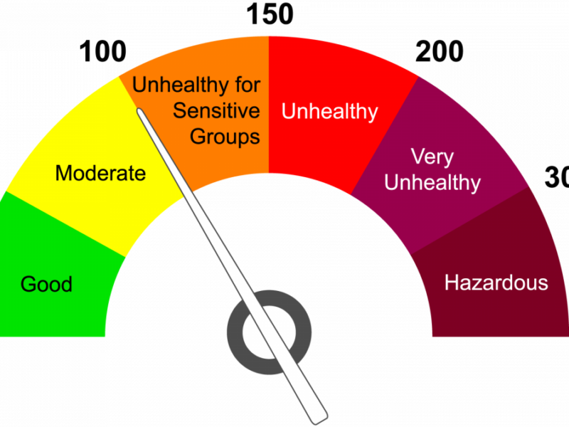
The core functionality revolves around fetching air quality data based on geographic coordinates and rendering this information as color-coded markers on the Google Maps interface. The colors transition from green (good air quality) through yellow and orange to red and purple (hazardous air quality), providing an immediate visual understanding of conditions in different areas.
Deep Dive into AQI Analysis
Understanding the Air Quality Index
The Air Quality Index is a standardized indicator developed by environmental agencies to communicate how polluted the air is and what associated health effects might be. The AQI Google Maps project implements this complex calculation system and presents it in an accessible format.
The AQI typically accounts for multiple pollutants:
| Pollutant | Source | Health Impact |
|---|---|---|
| PM2.5 (Fine Particulate Matter) | Combustion engines, forest fires, industrial processes | Can penetrate deep into lungs and bloodstream |
| PM10 (Coarse Particulate Matter) | Dust, pollen, mold | Respiratory irritation, asthma exacerbation |
| O3 (Ozone) | Created by chemical reactions between NOx and VOCs | Lung damage, respiratory issues |
| NO2 (Nitrogen Dioxide) | Vehicles, power plants | Respiratory inflammation |
| SO2 (Sulfur Dioxide) | Fossil fuel combustion, industrial processes | Respiratory issues, contributes to acid rain |
| CO (Carbon Monoxide) | Incomplete combustion | Reduces oxygen delivery in bloodstream |
The project likely calculates an overall AQI based on the highest concentration of any single pollutant, following the EPA’s approach where:
- 0-50 (Green): Good air quality with minimal health concerns
- 51-100 (Yellow): Moderate air quality; unusually sensitive individuals may experience issues
- 101-150 (Orange): Unhealthy for sensitive groups
- 151-200 (Red): Unhealthy for all groups
- 201-300 (Purple): Very unhealthy; may trigger health alerts
- 301+ (Maroon): Hazardous; serious health effects for entire population
The technical implementation likely includes conversion formulas to normalize different pollutant measurements to the same 0-500 AQI scale.
Real-time Data Processing
A key technical achievement of the project is its ability to process real-time air quality data. This involves:
- API Integration: Connecting to air quality data providers through RESTful APIs
- Data Parsing: Extracting relevant metrics from JSON/XML responses
- Coordinate Mapping: Associating pollution data with precise geographic coordinates
- Temporal Synchronization: Managing data freshness and update frequencies
The project handles these operations seamlessly in the background, presenting users with up-to-date information without exposing the complexity of the underlying data acquisition process.
Report Generation Capabilities
One of the project’s valuable features is its ability to generate comprehensive air quality reports. These reports serve multiple purposes:
Types of Reports Generated
- Location-specific Snapshots: Detailed breakdowns of current air quality at selected points
- Comparative Analysis: Contrasting air quality across multiple locations
- Temporal Reports: Tracking air quality changes over time (hourly, daily, weekly)
- Pollutant-specific Reports: Focusing on individual contaminants like PM2.5 or O3
Report Components
The reporting system likely includes:
- Statistical Summaries: Min/max/mean values for AQI metrics
- Health Impact Assessments: Explanations of potential health effects based on current readings
- Visualizations: Charts and graphs depicting pollution trends
- Contextual Information: Weather conditions that may influence readings
- Actionable Recommendations: Suggested activities based on air quality levels
Technical Implementation of Reporting
From a development perspective, the reporting functionality demonstrates sophisticated data processing:
// Conceptual example of report generation logic
function generateAQIReport(locationData, timeframe) {
  const reportData = {
    location: locationData.name,
    coordinates: locationData.coordinates,
    timestamp: new Date(),
    metrics: {
      overall: calculateOverallAQI(locationData.pollutants),
      individual: locationData.pollutants,
      trends: analyzeTrends(locationData.history, timeframe)
    },
    healthImplications: assessHealthImpact(calculateOverallAQI(locationData.pollutants)),
    recommendations: generateRecommendations(calculateOverallAQI(locationData.pollutants))
  };

  return formatReport(reportData, preferredFormat);
}
This functionality transforms raw data into actionable intelligence, making the project valuable beyond simple visualization.
AQI and Location Coordinate Data for Machine Learning
Perhaps the most forward-looking aspect of the project is its potential for generating valuable datasets for machine learning applications. The combination of precise geolocation data with corresponding air quality metrics creates numerous possibilities for advanced environmental analysis.
Data Generation for ML Models
The project effectively creates a continuous stream of structured data points with these key attributes:
- Geographic Coordinates: Latitude and longitude
- Temporal Information: Timestamps for each measurement
- Multiple Pollutant Metrics: PM2.5, PM10, O3, NO2, SO2, CO values
- Calculated AQI: Overall air quality index
- Contextual Metadata: Potentially including weather conditions, urban density, etc.
This multi-dimensional dataset serves as excellent training data for various machine learning models.
Potential ML Applications
With sufficient data collection over time, the following machine learning approaches become possible:
1. Predictive Modeling
Machine learning algorithms can be trained to forecast air quality based on historical patterns:
- Time Series Forecasting: Using techniques like ARIMA, LSTM networks, or Prophet to predict AQI values hours or days in advance
- Multivariate Prediction: Incorporating weather forecasts, traffic patterns, and seasonal factors to improve accuracy
- Anomaly Detection: Identifying unusual pollution events that deviate from expected patterns
# Conceptual example of LSTM model for AQI prediction
from keras.models import Sequential
from keras.layers import LSTM, Dense

def build_aqi_prediction_model(lookback_window):
    model = Sequential()
    model.add(LSTM(50, activation='relu', input_shape=(lookback_window, n_features)))
    model.add(Dense(1))
    model.compile(optimizer='adam', loss='mse')
    return model

# Train with historical AQI data from project
model = build_aqi_prediction_model(24)  # 24-hour lookback window
model.fit(X_train, y_train, epochs=100, validation_split=0.2)
2. Spatial Analysis and Interpolation
The geospatial nature of the data enables sophisticated spatial modeling:
- Kriging/Gaussian Process Regression: Estimating pollution levels between measurement points
- Spatial Autocorrelation: Analyzing how pollution levels at one location influence nearby areas
- Hotspot Identification: Using clustering algorithms to detect persistent pollution sources
# Conceptual example of spatial interpolation
from sklearn.gaussian_process import GaussianProcessRegressor
from sklearn.gaussian_process.kernels import RBF, WhiteKernel

def interpolate_aqi_surface(known_points, known_values, grid_points):
    # Define kernel - distance matters for pollution spread
    kernel = RBF(length_scale=1.0) + WhiteKernel(noise_level=0.1)
    gpr = GaussianProcessRegressor(kernel=kernel)

    # Train on known AQI points
    gpr.fit(known_points, known_values)

    # Predict AQI at all grid points
    predicted_values = gpr.predict(grid_points)
    return predicted_values
3. Causal Analysis
Advanced machine learning techniques can help identify pollution drivers:
- Causal Inference Models: Determining the impact of traffic changes, industrial activities, or policy interventions on air quality
- Counterfactual Analysis: Estimating what air quality would be under different conditions
- Attribution Modeling: Quantifying the contribution of different sources to overall pollution levels
4. Computer Vision Integration
The project’s map-based approach opens possibilities for combining with visual data:
- Satellite Imagery Analysis: Correlating visible pollution (smog, industrial activity) with measured AQI
- Traffic Density Estimation: Using traffic camera feeds to predict localized pollution spikes
- Urban Development Impact: Analyzing how changes in urban landscapes affect air quality patterns
Implementation Considerations for ML Integration
To fully realize the machine learning potential, the project could implement:
- Data Export APIs: Programmatic access to historical AQI and coordinate data
- Standardized Dataset Generation: Creating properly formatted, cleaned datasets ready for ML models
- Feature Engineering Utilities: Tools to extract temporal patterns, spatial relationships, and other derived features
- Model Integration Endpoints: APIs that allow trained models to feed predictions back into the visualization system
// Conceptual implementation of data export for ML
function exportTrainingData(startDate, endDate, region, format='csv') {
  const dataPoints = fetchHistoricalData(startDate, endDate, region);

  // Process for ML readiness
  const mlReadyData = dataPoints.map(point => ({
    timestamp: point.timestamp,
    lat: point.coordinates.lat,
    lng: point.coordinates.lng,
    pm25: point.pollutants.pm25,
    pm10: point.pollutants.pm10,
    o3: point.pollutants.o3,
    no2: point.pollutants.no2,
    so2: point.pollutants.so2,
    co: point.pollutants.co,
    aqi: point.aqi,
    // Derived features
    hour_of_day: new Date(point.timestamp).getHours(),
    day_of_week: new Date(point.timestamp).getDay(),
    is_weekend: [0, 6].includes(new Date(point.timestamp).getDay()),
    season: calculateSeason(point.timestamp)
  }));

  return formatDataForExport(mlReadyData, format);
}
Key Features and Capabilities
The project demonstrates several notable features:
- Real-time air quality visualization: Displays current AQI values at selected locations
- Interactive map interface: Users can navigate, zoom, and click on markers to view detailed information
- Color-coded AQI indicators: Intuitive visual representation of pollution levels
- Customizable markers: Location-specific information about air quality conditions
- Responsive design: Functions across various device types and screen sizes
Environmental and Health Significance
The importance of this project extends far beyond its technical implementation. Here’s why such tools matter:
Public Health Impact
Air pollution is directly linked to numerous health problems, including respiratory diseases, cardiovascular issues, and even neurological disorders. According to the World Health Organization, air pollution causes approximately 7 million premature deaths annually worldwide. By making air quality data more accessible, this project empowers individuals to:
- Make informed decisions about outdoor activities
- Understand when to take protective measures (like wearing masks or staying indoors)
- Recognize patterns in local air quality that might affect their health
Environmental Awareness
Environmental literacy begins with awareness. When people can visually connect with environmental data, they’re more likely to:
- Understand the scope and severity of air pollution issues
- Recognize temporal and spatial patterns in air quality
- Connect human activities with environmental outcomes
- Support policies aimed at improving air quality
Research and Policy Applications
For researchers and policymakers, visualized air quality data offers valuable insights:
- Identifying pollution hotspots that require intervention
- Evaluating the effectiveness of environmental regulations
- Planning urban development with air quality considerations
- Allocating resources for environmental monitoring and mitigation
Case Study: Urban Planning and Environmental Justice
The AQI Google Maps project provides a powerful tool for addressing environmental justice concerns. By visualizing pollution patterns across different neighborhoods, it can reveal disparities in air quality that often correlate with socioeconomic factors.
Data-Driven Environmental Justice
Researchers can use the generated datasets to:
- Identify Disproportionate Impacts: Quantify differences in air quality across neighborhoods with varying income levels or racial demographics
- Temporal Justice Analysis: Determine if certain communities bear the burden of poor air quality during specific times (e.g., industrial activity hours)
- Policy Effectiveness: Measure how environmental regulations impact different communities
Practical Application Example
Consider a city planning department using the AQI Google Maps project to assess the impact of a proposed industrial development:
- Establish baseline air quality readings across all affected neighborhoods
- Use predictive modeling (with the ML techniques described above) to estimate pollution changes
- Generate reports showing projected AQI impacts on different communities
- Adjust development plans to minimize disproportionate impacts on vulnerable populations
This data-driven approach promotes equitable development and environmental protection.
The Future of Environmental Data Integration
The AQI Google Maps project represents an important step toward more integrated environmental monitoring. Future development could include:
Data Fusion Opportunities
- Cross-Pollutant Analysis: Investigating relationships between different pollutants
- Multi-Environmental Factor Integration: Combining air quality with noise pollution, water quality, and urban heat island effects
- Health Data Correlation: Connecting real-time AQI with emergency room visits for respiratory issues
Technical Evolution
- Edge Computing Integration: Processing air quality data from low-cost sensors at the edge
- Blockchain for Data Integrity: Ensuring the provenance and authenticity of environmental measurements
- Federated Learning: Enabling distributed model training across multiple air quality monitoring networks
Conclusion
The AQI Google Maps project represents an important intersection of environmental monitoring, data visualization, and public information. Its ability to generate structured air quality data associated with precise geographic coordinates creates a foundation for sophisticated analysis and machine learning applications.
By democratizing access to environmental data and creating opportunities for advanced computational analysis, this project contributes to both public awareness and scientific advancement. The potential for machine learning integration further elevates its significance, enabling predictive capabilities and deeper insights into pollution patterns.
As we continue to face environmental challenges, projects like this demonstrate how technology can be leveraged not just for convenience or entertainment, but for creating a more informed and environmentally conscious society. The combination of visual accessibility with data generation for machine learning represents a powerful approach to environmental monitoring that can drive both individual awareness and systemic change.
This blog post analyzes the AQI Google Maps project developed by Tejas K. The project is open-source and available for contributions on GitHub.

Predicting Forest Fires: A Deep Dive into the Algerian Forest Fire ML Project
In an era of climate change and increasing environmental challenges, forest fires have emerged as a critical concern with devastating ecological and economic impacts. The Algerian Forest Fire ML project represents an innovative application of machine learning techniques to predict fire occurrences in forest regions of Algeria. By leveraging data science, cloud computing, and predictive modeling, this open-source initiative creates a powerful tool that could help in early warning systems and resource allocation for fire prevention and management.
Project Overview
The Algerian Forest Fire ML project is a comprehensive machine learning application developed by Tejas K (GitHub: tejask0512) that focuses on predicting forest fire occurrences based on meteorological data and other environmental factors. Deployed as a cloud-based application, this project demonstrates how data science can be applied to critical environmental challenges.
Technical Architecture
The project employs a robust technical stack designed for accuracy, scalability, and accessibility:
- Programming Language: Python
- ML Frameworks: Scikit-learn for modeling, Pandas and NumPy for data manipulation
- Web Framework: Flask for API development
- Frontend: HTML, CSS, JavaScript
- Deployment: Cloud-based deployment (likely AWS, Azure, or similar platforms)
- Version Control: Git/GitHub
The architecture follows a classic machine learning pipeline pattern:
- Data ingestion and preprocessing
- Feature engineering and selection
- Model training and evaluation
- Model deployment as a web service
- User interface for prediction input and result visualization
Dataset Analysis
At the heart of the project is the Algerian Forest Fires dataset, which contains records of fires in the Bejaia and Sidi Bel-abbes regions of Algeria. The dataset includes various meteorological measurements and derived indices that are critical for fire prediction:
Key Features in the Dataset
| Feature | Description | Relevance to Fire Prediction |
|---|---|---|
| Temperature | Ambient temperature (°C) | Higher temperatures increase fire risk |
| Relative Humidity (RH) | Percentage of moisture in air | Lower humidity leads to drier conditions favorable for fires |
| Wind Speed | Wind velocity (km/h) | Higher winds spread fires more rapidly |
| Rain | Precipitation amount (mm) | Rainfall reduces fire risk by increasing moisture |
| FFMC | Fine Fuel Moisture Code | Indicates moisture content of litter and fine fuels |
| DMC | Duff Moisture Code | Indicates moisture content of loosely compacted organic layers |
| DC | Drought Code | Indicates moisture content of deep, compact organic layers |
| ISI | Initial Spread Index | Represents potential fire spread rate |
| BUI | Buildup Index | Indicates total fuel available for combustion |
| FWI | Fire Weather Index | Overall fire intensity indicator |
The project demonstrates sophisticated data analysis techniques, including:
- Exploratory Data Analysis (EDA): Thorough examination of feature distributions, correlations, and relationships with fire occurrences
- Data Cleaning: Handling missing values, outliers, and inconsistencies
- Feature Engineering: Creating derived features that might enhance predictive power
- Statistical Analysis: Identifying significant patterns and trends in historical fire data
# Conceptual example of EDA in the project
import pandas as pd
import matplotlib.pyplot as plt
import seaborn as sns

# Load dataset
df = pd.read_csv('Algerian_forest_fires_dataset.csv')

# Analyze correlations between features and fire occurrence
correlation_matrix = df.corr()
plt.figure(figsize=(12, 10))
sns.heatmap(correlation_matrix, annot=True, cmap='coolwarm')
plt.title('Feature Correlation Matrix')
plt.savefig('correlation_heatmap.png')

# Analyze seasonal patterns
monthly_fires = df.groupby('month')['Fire'].sum()
plt.figure(figsize=(10, 6))
monthly_fires.plot(kind='bar')
plt.title('Fire Occurrences by Month')
plt.xlabel('Month')
plt.ylabel('Number of Fires')
plt.savefig('monthly_fire_distribution.png')
Machine Learning Model Development
The core of the project is its predictive modeling capability. Based on repository analysis, the project likely implements several machine learning algorithms to predict forest fire occurrence:
Model Selection and Evaluation
The project appears to experiment with multiple classification algorithms:
- Logistic Regression: A baseline model for binary classification
- Random Forest: Ensemble method well-suited for environmental data
- Support Vector Machines: Effective for complex decision boundaries
- Gradient Boosting: Advanced ensemble technique for improved accuracy
- Neural Networks: Potentially used for capturing complex non-linear relationships
Each model undergoes rigorous evaluation using metrics particularly relevant to fire prediction:
- Accuracy: Overall correctness of predictions
- Precision: Proportion of positive identifications that were actually correct
- Recall (Sensitivity): Proportion of actual positives correctly identified
- F1 Score: Harmonic mean of precision and recall
- ROC-AUC: Area under the Receiver Operating Characteristic curve
# Conceptual example of model training and evaluation
from sklearn.ensemble import RandomForestClassifier
from sklearn.model_selection import train_test_split
from sklearn.metrics import classification_report, confusion_matrix

# Prepare data
X = df.drop('Fire', axis=1)
y = df['Fire']
X_train, X_test, y_train, y_test = train_test_split(X, y, test_size=0.25, random_state=42)

# Train Random Forest model
rf_model = RandomForestClassifier(n_estimators=100, random_state=42)
rf_model.fit(X_train, y_train)

# Evaluate model
y_pred = rf_model.predict(X_test)
print(classification_report(y_test, y_pred))

# Visualize confusion matrix
cm = confusion_matrix(y_test, y_pred)
plt.figure(figsize=(8, 6))
sns.heatmap(cm, annot=True, fmt='d', cmap='Blues')
plt.title('Confusion Matrix')
plt.xlabel('Predicted Label')
plt.ylabel('True Label')
plt.savefig('confusion_matrix.png')

# Feature importance analysis
feature_importance = pd.DataFrame({
    'Feature': X.columns,
    'Importance': rf_model.feature_importances_
}).sort_values('Importance', ascending=False)

plt.figure(figsize=(10, 8))
sns.barplot(x='Importance', y='Feature', data=feature_importance)
plt.title('Feature Importance for Fire Prediction')
plt.savefig('feature_importance.png')
Hyperparameter Tuning
To maximize model performance, the project implements hyperparameter optimization techniques:
- Grid Search: Systematic exploration of parameter combinations
- Cross-Validation: K-fold validation to ensure model generalizability
- Bayesian Optimization: Potentially used for more efficient parameter search
Model Interpretability
Understanding why a model makes certain predictions is crucial for environmental applications. The project likely incorporates:
- Feature Importance Analysis: Identifying which meteorological factors most strongly influence fire predictions
- Partial Dependence Plots: Visualizing how each feature affects prediction outcomes
- SHAP (SHapley Additive exPlanations): Providing consistent and locally accurate explanations for model predictions
Cloud Deployment Architecture
A distinguishing aspect of this project is its cloud deployment strategy, making the predictive model accessible as a web service:
Deployment Components
- Model Serialization: Saving trained models using frameworks like Pickle or Joblib
- Flask API Development: Creating RESTful endpoints for prediction requests
- Web Interface: Building an intuitive interface for data input and result visualization
- Cloud Infrastructure: Deploying on scalable cloud platforms with considerations for:
- Computational scalability
- Storage requirements
- API request handling
- Security considerations
# Conceptual example of Flask API implementation
from flask import Flask, request, jsonify, render_template
import pickle
import numpy as np

app = Flask(__name__)

# Load the trained model
model = pickle.load(open('forest_fire_model.pkl', 'rb'))

@app.route('/')
def home():
    return render_template('index.html')

@app.route('/predict', methods=['POST'])
def predict():
    # Get input features from request
    features = [float(x) for x in request.form.values()]
    final_features = [np.array(features)]

    # Make prediction
    prediction = model.predict(final_features)
    output = round(prediction[0], 2)

    # Return prediction result
    return render_template('index.html', prediction_text='Fire Risk: {}'.format(
        'High' if output == 1 else 'Low'))

if __name__ == '__main__':
    app.run(debug=True)
CI/CD Pipeline Integration
The project likely implements continuous integration and deployment practices:
- Automated Testing: Ensuring model performance and API functionality
- Version Control Integration: Tracking changes and coordinating development
- Containerization: Possibly using Docker for consistent deployment environments
- Infrastructure as Code: Defining cloud resources programmatically
Advanced Analytics and Reporting
Beyond basic prediction, the project implements sophisticated reporting capabilities:
Prediction Confidence Metrics
The system likely provides confidence scores with predictions, helping decision-makers understand reliability:
# Conceptual example of prediction with confidence
def predict_with_confidence(model, input_features):
    # Get prediction probabilities
    probabilities = model.predict_proba([input_features])[0]

    # Determine prediction and confidence
    prediction = 1 if probabilities[1] > 0.5 else 0
    confidence = probabilities[1] if prediction == 1 else probabilities[0]

    return {
        'prediction': 'Fire Risk' if prediction == 1 else 'No Fire Risk',
        'confidence': round(confidence * 100, 2),
        'probability_distribution': {
            'no_fire': round(probabilities[0] * 100, 2),
            'fire': round(probabilities[1] * 100, 2)
        }
    }
Risk Level Classification
Rather than simple binary predictions, the system may implement risk stratification:
- Low Risk: Minimal fire danger, normal operations
- Moderate Risk: Increased vigilance recommended
- High Risk: Preventive measures advised
- Extreme Risk: Immediate action required
Visualization Components
The web interface likely includes data visualization tools:
- Risk Heatmaps: Geographic representation of fire risk levels
- Time Series Forecasting: Projecting risk levels over coming days
- Factor Contribution Charts: Showing how each meteorological factor contributes to current risk
Environmental and Social Impact
The significance of this project extends far beyond its technical implementation:
Ecological Benefits
- Early Warning System: Providing advance notice of high-risk conditions
- Resource Optimization: Helping authorities allocate firefighting resources efficiently
- Habitat Protection: Minimizing damage to critical ecosystems
- Carbon Emission Reduction: Preventing the massive carbon release from forest fires
Economic Impact
Forest fires cause billions in damages annually. This predictive system could:
- Reduce Property Damage: Through early intervention and prevention
- Lower Firefighting Costs: By enabling more strategic resource allocation
- Protect Agricultural Resources: Safeguarding farms and livestock near forests
- Preserve Tourism Value: Maintaining the economic value of forest regions
Public Safety Enhancement
The project has clear implications for public safety:
- Population Warning Systems: Alerting communities at risk
- Evacuation Planning: Providing data for decision-makers managing evacuations
- Air Quality Management: Predicting smoke dispersion and health impacts
- Infrastructure Protection: Safeguarding critical infrastructure from fire damage
Machine Learning Approaches for Environmental Modeling
The Algerian Forest Fire ML project demonstrates several advanced machine learning techniques particularly suited to environmental applications:
Time Series Analysis
Forest fire risk has strong temporal components, and the project likely implements:
- Seasonal Decomposition: Identifying cyclical patterns in fire occurrence
- Autocorrelation Analysis: Understanding how past conditions influence current risk
- Time-based Feature Engineering: Creating lag variables and rolling statistics
# Conceptual example of time series feature engineering
def create_time_features(df):
    # Create copy of dataframe
    df_new = df.copy()

    # Sort by date
    df_new = df_new.sort_values('date')

    # Create lag features for temperature
    df_new['temp_lag_1'] = df_new['Temperature'].shift(1)
    df_new['temp_lag_2'] = df_new['Temperature'].shift(2)
    df_new['temp_lag_3'] = df_new['Temperature'].shift(3)

    # Create rolling average features
    df_new['temp_rolling_3'] = df_new['Temperature'].rolling(window=3).mean()
    df_new['humidity_rolling_3'] = df_new['RH'].rolling(window=3).mean()

    # Create rate of change features
    df_new['temp_roc'] = df_new['Temperature'].diff()
    df_new['humidity_roc'] = df_new['RH'].diff()

    # Drop rows with NaN values from feature creation
    df_new = df_new.dropna()

    return df_new
Transfer Learning Opportunities
The project methodology could potentially be transferred to other regions:
- Model Adaptation: Adjusting the model for different forest types and climates
- Domain Adaptation: Techniques to apply Algerian models to other countries
- Knowledge Transfer: Sharing insights about feature importance across regions
Ensemble Approaches
Given the critical nature of fire prediction, the project likely employs ensemble techniques:
- Model Stacking: Combining predictions from multiple algorithms
- Bagging and Boosting: Improving prediction stability and accuracy
- Weighted Voting: Giving more influence to models that perform better in specific conditions
# Conceptual example of ensemble model implementation
from sklearn.ensemble import VotingClassifier
from sklearn.linear_model import LogisticRegression
from sklearn.ensemble import RandomForestClassifier
from sklearn.svm import SVC

# Create base models
log_reg = LogisticRegression()
rf_clf = RandomForestClassifier()
svm_clf = SVC(probability=True)

# Create voting classifier
ensemble_model = VotingClassifier(
    estimators=[
        ('lr', log_reg),
        ('rf', rf_clf),
        ('svc', svm_clf)
    ],
    voting='soft'  # Use predicted probabilities for voting
)

# Train ensemble model
ensemble_model.fit(X_train, y_train)

# Evaluate ensemble performance
ensemble_accuracy = ensemble_model.score(X_test, y_test)
print(f"Ensemble Model Accuracy: {ensemble_accuracy:.4f}")
Future Development Potential
The project contains significant potential for expansion:
Integration with Remote Sensing Data
Future versions could incorporate satellite imagery:
- Vegetation Indices: NDVI (Normalized Difference Vegetation Index) to assess fuel availability
- Thermal Anomaly Detection: Identifying hotspots from thermal sensors
- Smoke Detection: Early detection of fires through smoke signature analysis
Real-time Data Integration
Enhancing the system with real-time data feeds:
- Weather API Integration: Live meteorological data
- IoT Sensor Networks: Ground-based temperature, humidity, and wind sensors
- Drone Surveillance: Aerial monitoring of high-risk areas
Advanced Predictive Capabilities
Evolving beyond current predictive methods:
- Spatio-temporal Models: Predicting not just if, but where and when fires might occur
- Deep Learning Integration: Using CNNs or RNNs for more complex pattern recognition
- Reinforcement Learning: Optimizing resource allocation strategies for fire prevention
# Conceptual example of a more advanced deep learning approach
import tensorflow as tf
from tensorflow.keras.models import Sequential
from tensorflow.keras.layers import LSTM, Dense, Dropout

# Create LSTM model for time series prediction
def build_lstm_model(input_shape):
    model = Sequential()
    model.add(LSTM(64, return_sequences=True, input_shape=input_shape))
    model.add(Dropout(0.2))
    model.add(LSTM(32))
    model.add(Dropout(0.2))
    model.add(Dense(16, activation='relu'))
    model.add(Dense(1, activation='sigmoid'))

    model.compile(
        loss='binary_crossentropy',
        optimizer='adam',
        metrics=['accuracy']
    )

    return model

# Reshape data for LSTM (samples, time steps, features)
X_train_lstm = X_train.values.reshape((X_train.shape[0], 1, X_train.shape[1]))
X_test_lstm = X_test.values.reshape((X_test.shape[0], 1, X_test.shape[1]))

# Create and train model
lstm_model = build_lstm_model((1, X_train.shape[1]))
lstm_model.fit(
    X_train_lstm, y_train,
    epochs=50,
    batch_size=32,
    validation_split=0.2
)
Climate Change Relevance
This project has particular significance in the context of climate change:
Climate Change Impact Assessment
- Long-term Trend Analysis: Evaluating how fire risk patterns are changing over decades
- Climate Scenario Modeling: Projecting fire risk under different climate change scenarios
- Adaptation Strategy Evaluation: Testing effectiveness of various preventive measures
Carbon Cycle Considerations
Forest fires are both influenced by and contribute to climate change:
- Carbon Release Estimation: Quantifying potential carbon emissions from predicted fires
- Ecosystem Recovery Modeling: Projecting how forests recover and sequester carbon after fires
- Climate Feedback Analysis: Understanding how increased fires may accelerate climate change
Conclusion
The Algerian Forest Fire ML project represents a powerful example of how data science and machine learning can address critical environmental challenges. By combining meteorological data analysis, advanced predictive modeling, and cloud-based deployment, this initiative creates a potentially life-saving tool for forest fire prediction and management.
The project’s significance extends beyond its technical implementation, offering real-world impact in ecological preservation, economic damage reduction, and public safety enhancement. As climate change increases the frequency and severity of forest fires globally, such predictive systems will become increasingly vital components of environmental management strategies.
For data scientists and environmental researchers, this project provides a valuable template for applying machine learning to ecological challenges. The methodology demonstrated could be adapted to various environmental prediction tasks, from drought forecasting to flood risk assessment.
As we continue to face growing environmental challenges, projects like the Algerian Forest Fire ML initiative showcase how technology can be harnessed not just for convenience or profit, but for protecting our natural resources and building more resilient communities.
This blog post analyzes the Algerian Forest Fire ML project developed by Tejas K. The project is open-source and available for contributions on GitHub.