
Recurrent Neural Networks
Humans don’t begin their thought process from zero every moment. As you read this essay, you interpret each word in the context of the ones that came before it. You don’t discard everything and restart your thinking each time — your thoughts carry forward.
Conventional neural networks lack this ability, which is a significant limitation. For instance, if you’re trying to identify what type of event is occurring at each moment in a movie, a traditional neural network struggles to incorporate knowledge of earlier scenes to make sense of later ones.
Recurrent neural networks (RNNs) overcome this limitation. These networks are designed with loops that allow information to be retained over time, enabling them to maintain context.
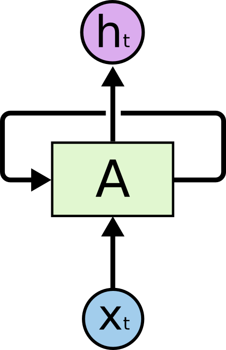
Recurrent Neural Networks have loops.
In the above diagram, a chunk of neural network, AA, looks at some input XtXt and outputs a value htht. A loop allows information to be passed from one step of the network to the next.
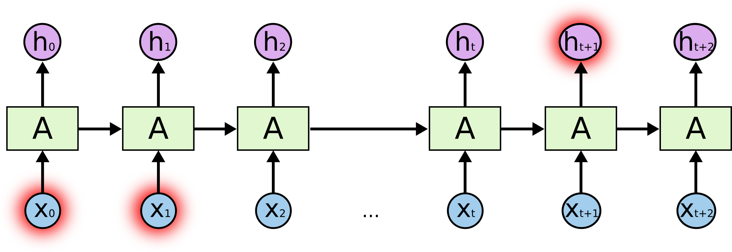
These loops make recurrent neural networks seem kind of mysterious. However, if you think a bit more, it turns out that they aren’t all that different than a normal neural network. A recurrent neural network can be thought of as multiple copies of the same network, each passing a message to a successor. Consider what happens if we unroll the loop:
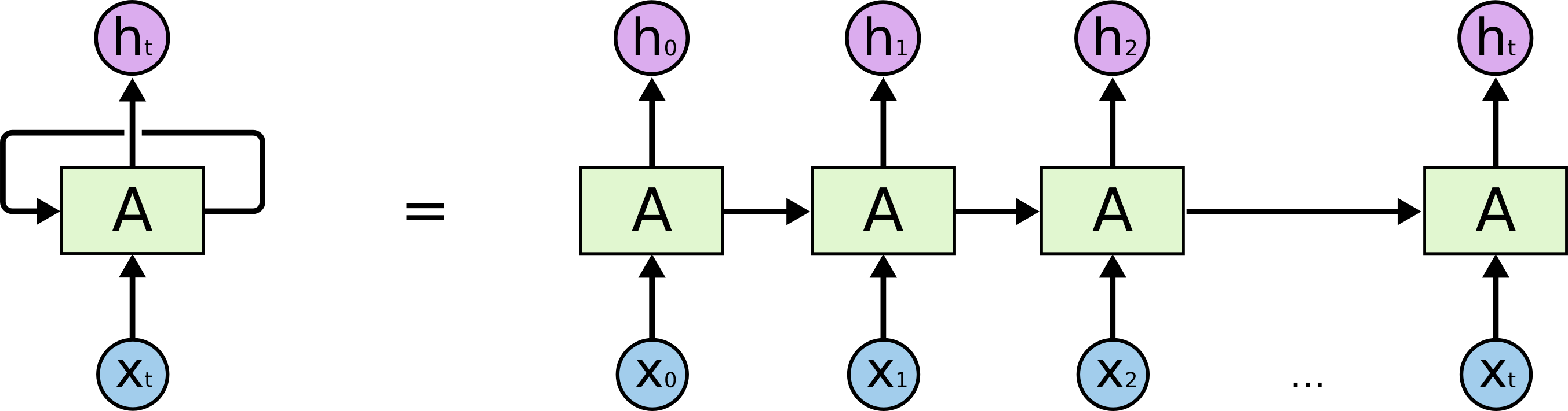
An unrolled recurrent neural network.
The chain-like structure of recurrent neural networks (RNNs) makes them naturally suited for handling sequential data, such as lists and time series. They’re the go-to neural network architecture for this kind of information.
And indeed, they’ve been widely adopted! In recent years, RNNs have driven remarkable progress in fields like speech recognition, language modeling, translation, image captioning, and more.
A major factor behind these achievements is the use of LSTMs — a specialized type of RNN that outperforms the standard model on many tasks. Most of the exciting advancements involving RNNs have been made possible thanks to LSTMs, and this essay will focus on exploring how they work.
The Problem of Long-Term Dependencies
One of the appeals of RNNs is the idea that they might be able to connect previous information to the present task, such as using previous video frames might inform the understanding of the present frame. If RNNs could do this, they’d be extremely useful. But can they? It depends.
Sometimes, we only need to look at recent information to perform the present task. For example, consider a language model trying to predict the next word based on the previous ones. If we are trying to predict the last word in “the clouds are in the sky,” we don’t need any further context – it’s pretty obvious the next word is going to be sky. In such cases, where the gap between the relevant information and the place that it’s needed is small, RNNs can learn to use the past information.
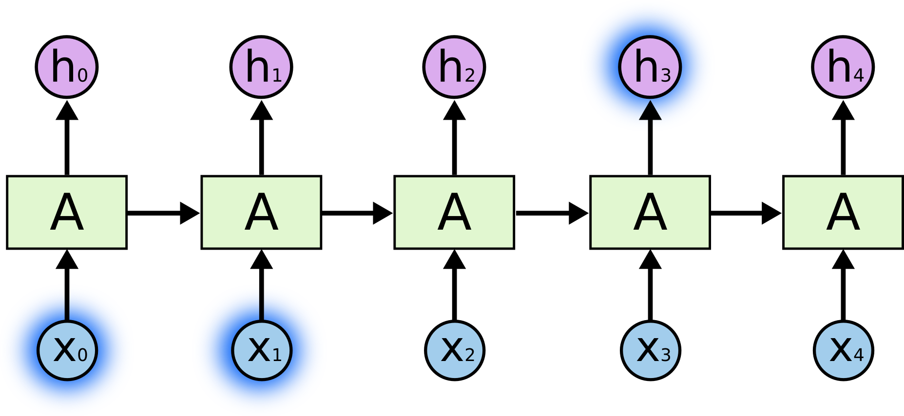
But there are also cases where we need more context. Consider trying to predict the last word in the text “I grew up in France… I speak fluent French.” Recent information suggests that the next word is probably the name of a language, but if we want to narrow down which language, we need the context of France, from further back. It’s entirely possible for the gap between the relevant information and the point where it is needed to become very large.
Unfortunately, as that gap grows, RNNs become unable to learn to connect the information.
In theory, RNNs are absolutely capable of handling such “long-term dependencies.” A human could carefully pick parameters for them to solve toy problems of this form. Sadly, in practice, RNNs don’t seem to be able to learn them. The problem was explored in depth by Hochreiter (1991) [German] and Bengio, et al. (1994), who found some pretty fundamental reasons why it might be difficult.
Thankfully, LSTMs don’t have this problem!
LSTM Networks
Long Short-Term Memory networks, or simply LSTMs, are a specialized type of recurrent neural network (RNN) designed to learn and retain information over long sequences. First introduced by Hochreiter and Schmidhuber in 1997, they’ve since been improved and widely adopted due to their impressive performance across a broad range of tasks.
LSTMs are specifically built to overcome the challenge of long-term dependencies in sequence modeling. While standard RNNs often struggle to retain information across many time steps, LSTMs are inherently capable of doing so — maintaining relevant information over long periods is a core part of how they function.
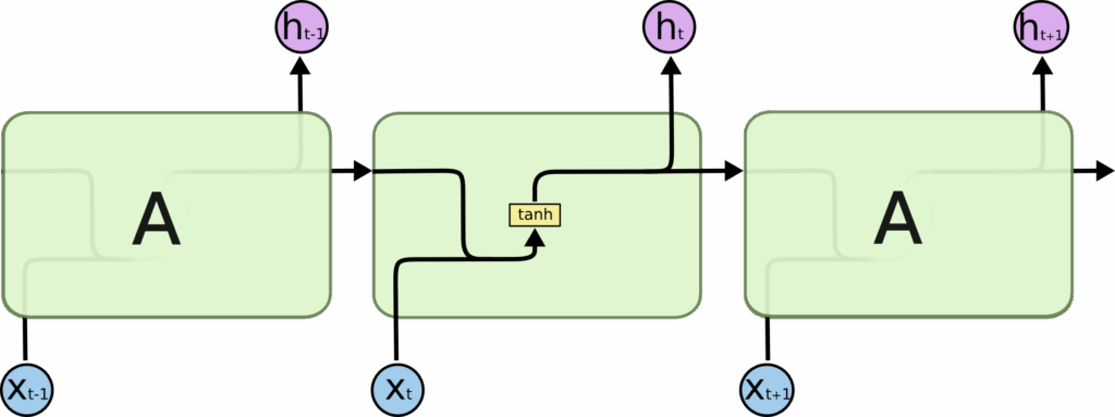
Like all RNNs, LSTMs consist of a chain of repeating neural network modules. However, while a basic RNN typically uses a simple structure like a single tanh layer in each module, LSTMs replace this with a more sophisticated internal architecture designed to preserve and control information flow more effectively.
The Word1 Xt-1 sent to the neural network, then word2 is sent to the neural network , Xt-1 is provided as input to calculate ht, we calculate Cosine Similarity Between the Words to check the relation between them, with respect to the features.
The repeating module in a standard RNN contains a single layer.
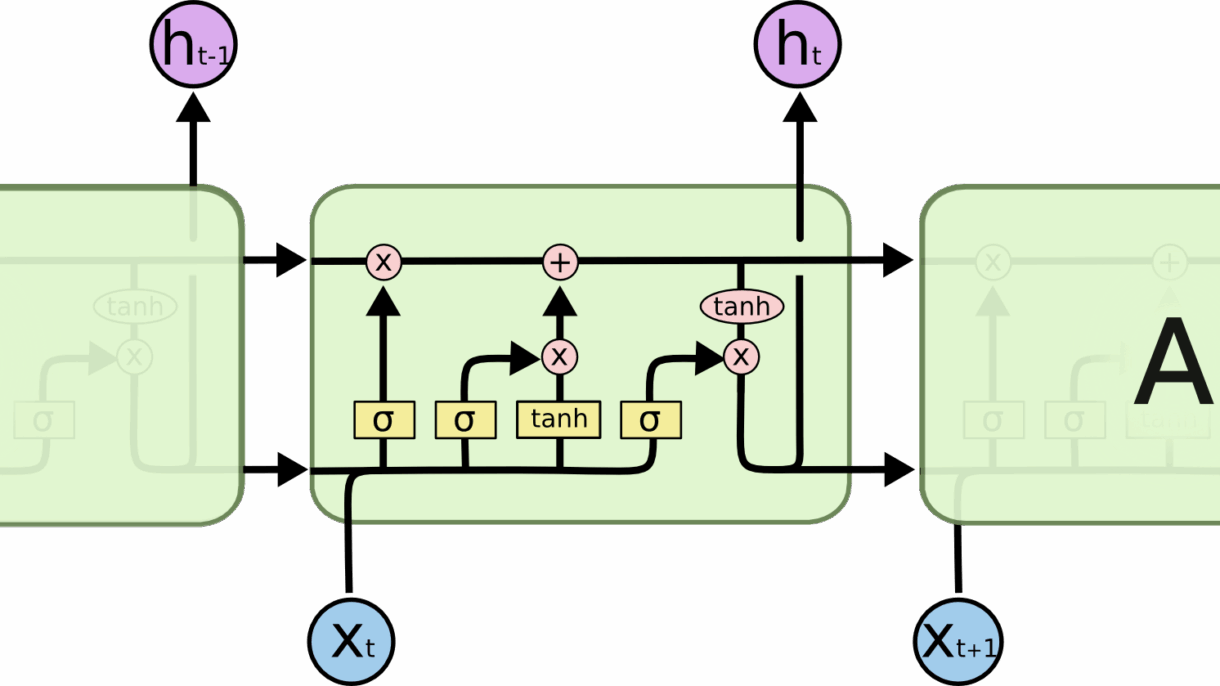
LSTMs also have this chain like structure, but the repeating module has a different structure. Instead of having a single neural network layer, there are four, interacting in a very special way.
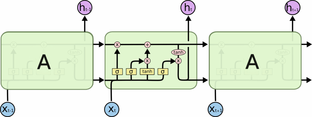
The repeating module in an LSTM contains four interacting layers.
Don’t worry about the details of what’s going on. We’ll walk through the LSTM diagram step by step later. For now, let’s just try to get comfortable with the notation we’ll be using.
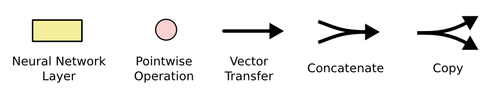
In the above diagram, each line carries an entire vector, from the output of one node to the inputs of others. The pink circles represent pointwise operations, like vector addition, while the yellow boxes are learned neural network layers. Lines merging denote concatenation, while a line forking denote its content being copied and the copies going to different locations.
The Core Idea Behind LSTMs
The key to LSTMs is the cell state, the horizontal line running through the top of the diagram.
The cell state is kind of like a conveyor belt. It runs straight down the entire chain, with only some minor linear interactions. It’s very easy for information to just flow along it unchanged.
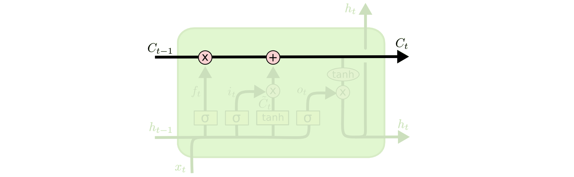
The LSTM does have the ability to remove or add information to the cell state, carefully regulated by structures called gates.
Gates are a way to optionally let information through. They are composed out of a sigmoid neural net layer and a pointwise multiplication operation.
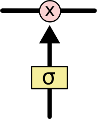
The sigmoid layer outputs numbers between zero and one, describing how much of each component should be let through. A value of zero means “let nothing through,” while a value of one means “let everything through!”
An LSTM has three of these gates, to protect and control the cell state.
Step-by-Step LSTM Walk Through
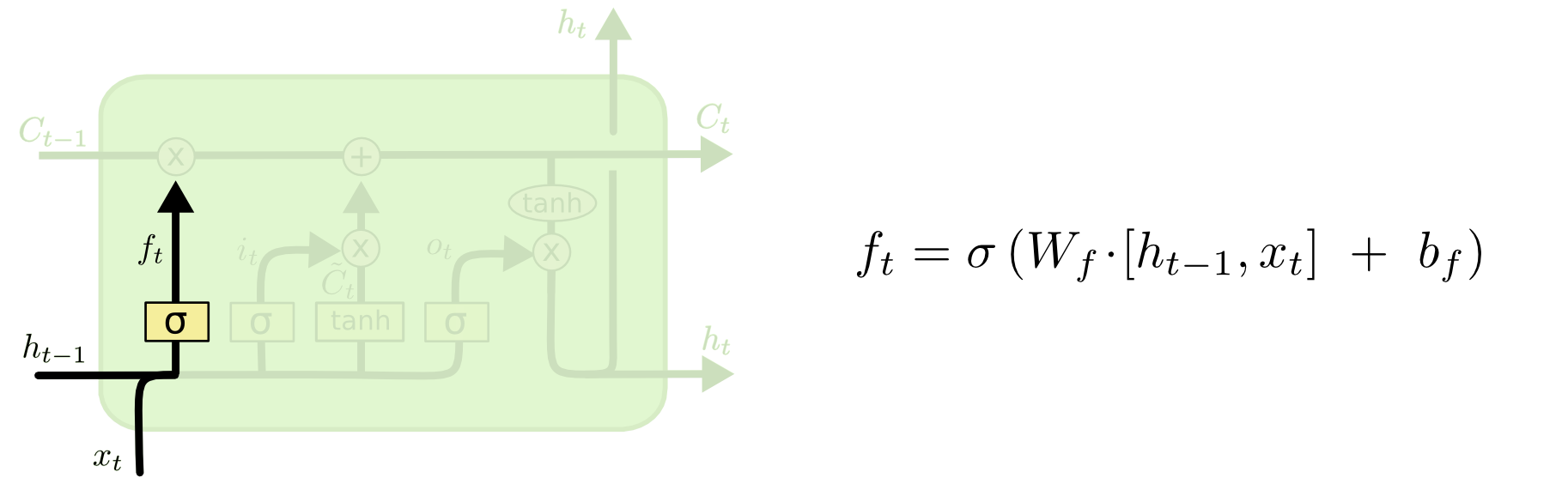
The first step in our LSTM is to decide what information we’re going to throw away from the cell state. This decision is made by a sigmoid layer called the “forget gate layer.” It looks at ht−1ht−1 and xtxt, and outputs a number between 00 and 11 for each number in the cell state Ct−1Ct−1. A 11 represents “completely keep this” while a 00 represents “completely get rid of this.”
Let’s go back to our example of a language model trying to predict the next word based on all the previous ones. In such a problem, the cell state might include the gender of the present subject, so that the correct pronouns can be used. When we see a new subject, we want to forget the gender of the old subject.
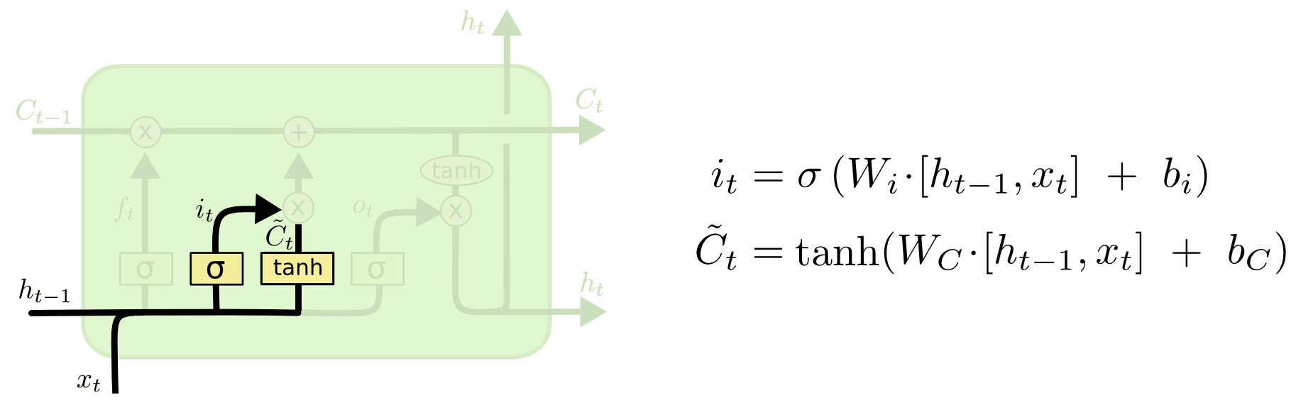
The next step is to decide what new information we’re going to store in the cell state. This has two parts. First, a sigmoid layer called the “input gate layer” decides which values we’ll update. Next, a tanh layer creates a vector of new candidate values, C~tC~t, that could be added to the state. In the next step, we’ll combine these two to create an update to the state.
In the example of our language model, we’d want to add the gender of the new subject to the cell state, to replace the old one we’re forgetting.
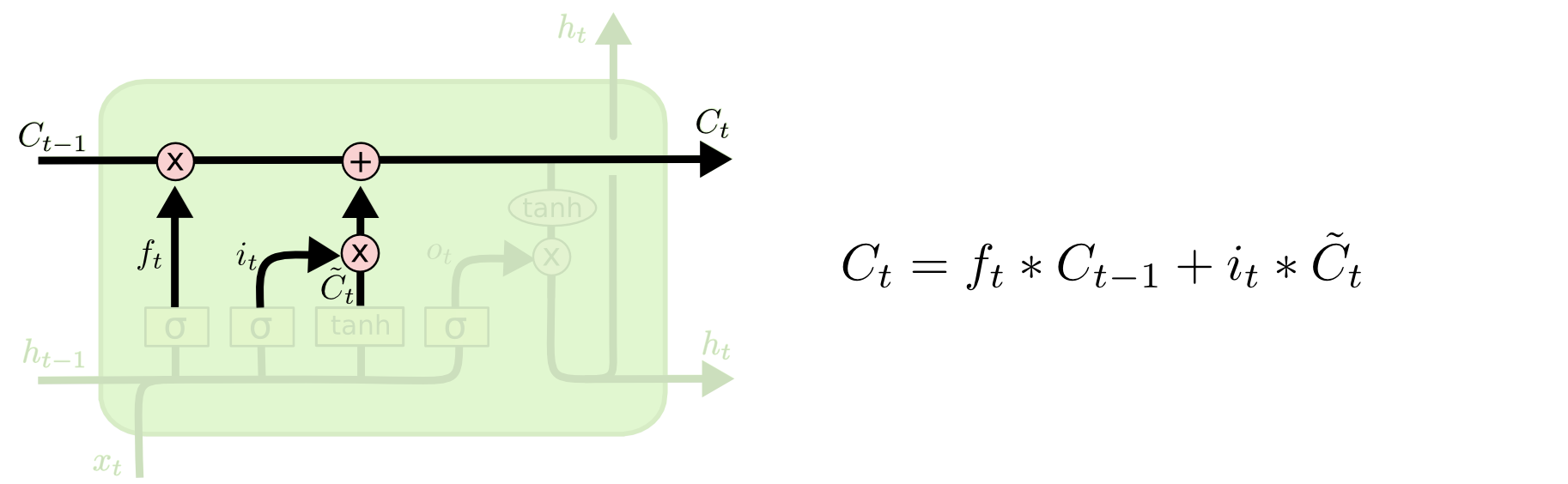
It’s now time to update the old cell state, Ct−1Ct−1, into the new cell state CtCt. The previous steps already decided what to do, we just need to actually do it.
We multiply the old state by ftft, forgetting the things we decided to forget earlier. Then we add it∗C~tit∗C~t. This is the new candidate values, scaled by how much we decided to update each state value.
In the case of the language model, this is where we’d actually drop the information about the old subject’s gender and add the new information, as we decided in the previous steps.
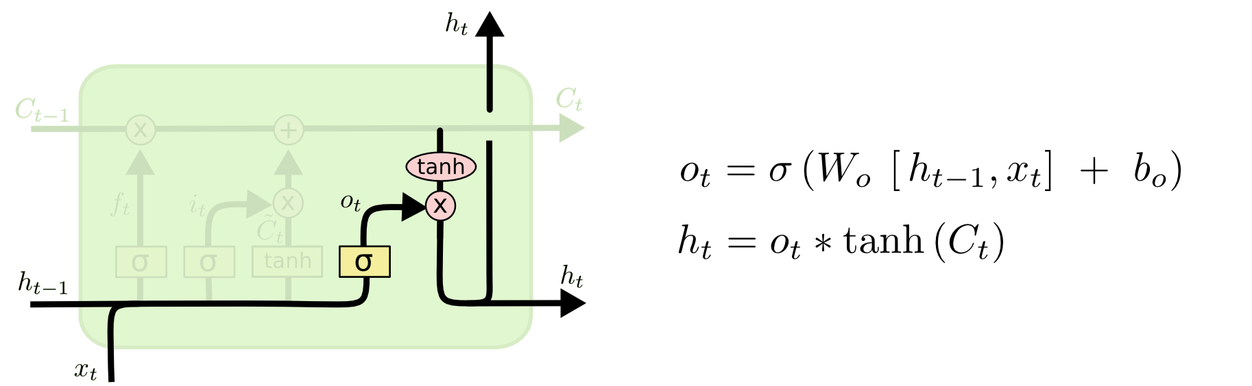
Finally, we need to decide what we’re going to output. This output will be based on our cell state, but will be a filtered version. First, we run a sigmoid layer which decides what parts of the cell state we’re going to output. Then, we put the cell state through tanhtanh (to push the values to be between −1−1 and 11) and multiply it by the output of the sigmoid gate, so that we only output the parts we decided to.
For the language model example, since it just saw a subject, it might want to output information relevant to a verb, in case that’s what is coming next. For example, it might output whether the subject is singular or plural, so that we know what form a verb should be conjugated into if that’s what follows next.
Variants on Long Short Term Memory
What I’ve described so far is a pretty normal LSTM. But not all LSTMs are the same as the above. In fact, it seems like almost every paper involving LSTMs uses a slightly different version. The differences are minor, but it’s worth mentioning some of them.
One popular LSTM variant, introduced by Gers & Schmidhuber (2000), is adding “peephole connections.” This means that we let the gate layers look at the cell state.
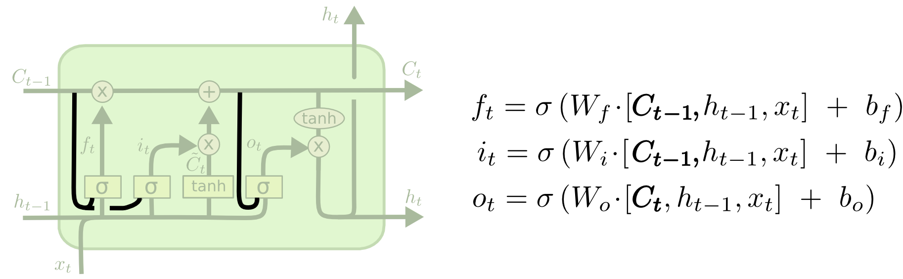
The above diagram adds peepholes to all the gates, but many papers will give some peepholes and not others.
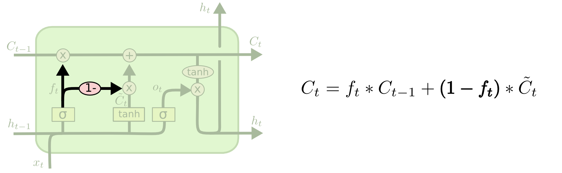
Another variation is to use coupled forget and input gates. Instead of separately deciding what to forget and what we should add new information to, we make those decisions together. We only forget when we’re going to input something in its place. We only input new values to the state when we forget something older.
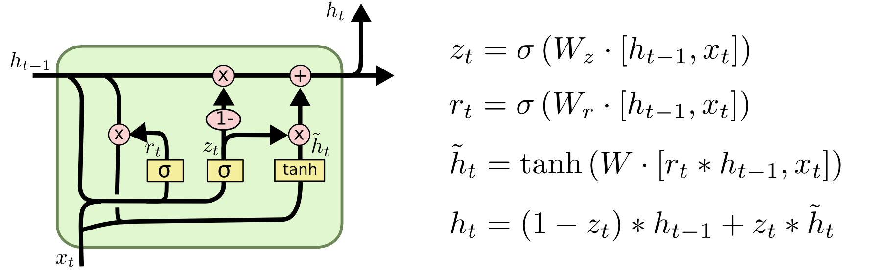
A slightly more dramatic variation on the LSTM is the Gated Recurrent Unit, or GRU, introduced by Cho, et al. (2014). It combines the forget and input gates into a single “update gate.” It also merges the cell state and hidden state, and makes some other changes. The resulting model is simpler than standard LSTM models, and has been growing increasingly popular.
These are only a few of the most notable LSTM variants. There are lots of others, like Depth Gated RNNs by Yao, et al. (2015). There’s also some completely different approach to tackling long-term dependencies, like Clockwork RNNs by Koutnik, et al. (2014).
Which of these variants is best? Do the differences matter? Greff, et al. (2015) do a nice comparison of popular variants, finding that they’re all about the same. Jozefowicz, et al. (2015) tested more than ten thousand RNN architectures, finding some that worked better than LSTMs on certain tasks.
Understanding RNN and LSTM: Forward and Backpropagation
Recurrent Neural Networks (RNNs) and Long Short-Term Memory networks (LSTMs) are fundamental architectures for sequence modeling in deep learning. This article provides a comprehensive mathematical foundation for both, including forward pass computations and the crucial backpropagation through time (BPTT) formulas for training.
1. Vanilla Recurrent Neural Networks (RNNs)
1.1 Forward Propagation
The standard RNN computes a sequence of hidden states and outputs from an input sequence:
For time step \(t\):
\begin{align} h_t &= \tanh(W_{hh} h_{t-1} + W_{xh} x_t + b_h) \\ y_t &= W_{hy} h_t + b_y \end{align}Where:
- \(x_t\) is the input at time step \(t\)
- \(h_t\) is the hidden state at time step \(t\)
- \(y_t\) is the output at time step \(t\)
- \(W_{xh}\) is the weight matrix from input to hidden layer
- \(W_{hh}\) is the recurrent weight matrix from hidden to hidden layer
- \(W_{hy}\) is the weight matrix from hidden to output layer
- \(b_h\) and \(b_y\) are bias vectors
- \(\tanh\) is the hyperbolic tangent activation function
1.2 Backpropagation Through Time (BPTT)
For a loss function \(L\) (typically cross-entropy for classification or mean squared error for regression), the gradients are:
Where \(\text{diag}(1 – h_{t+1}^2)\) represents the derivative of \(\tanh\) evaluated at the pre-activation values.
Note on the Vanishing/Exploding Gradient Problem: The recursion in calculating \(\frac{\partial L}{\partial h_t}\) involves multiplying by \(W_{hh}^T\) repeatedly, which can cause gradients to either vanish or explode during backpropagation through many time steps. This is a fundamental limitation of vanilla RNNs that LSTMs were designed to address.
2. Long Short-Term Memory Networks (LSTMs)
2.1 Forward Propagation
LSTMs introduce gating mechanisms to control information flow:
For time step \(t\):
\begin{align} f_t &= \sigma(W_f \cdot [h_{t-1}, x_t] + b_f) \\ i_t &= \sigma(W_i \cdot [h_{t-1}, x_t] + b_i) \\ \tilde{C}_t &= \tanh(W_C \cdot [h_{t-1}, x_t] + b_C) \\ C_t &= f_t \odot C_{t-1} + i_t \odot \tilde{C}_t \\ o_t &= \sigma(W_o \cdot [h_{t-1}, x_t] + b_o) \\ h_t &= o_t \odot \tanh(C_t) \\ y_t &= W_{hy} h_t + b_y \end{align}Where:
- \(f_t\) is the forget gate, determining what to discard from the cell state
- \(i_t\) is the input gate, determining what new information to store
- \(\tilde{C}_t\) is the candidate cell state
- \(C_t\) is the cell state
- \(o_t\) is the output gate
- \(h_t\) is the hidden state
- \(y_t\) is the output
- \([h_{t-1}, x_t]\) represents the concatenation of \(h_{t-1}\) and \(x_t\)
- \(\odot\) represents element-wise multiplication
- \(\sigma\) is the sigmoid activation function
2.2 Backpropagation Through Time for LSTMs
LSTM backpropagation is more complex due to the multiple gates and pathways. Here are the key derivatives:
For the hidden state backpropagation:
For the cell state candidate and gates:
Then, for the weight matrices:
And for the bias terms:
3. Practical Implementation Considerations
3.1 Gradient Clipping
To mitigate exploding gradients, a common practice is to clip gradients when their norm exceeds a threshold:
\begin{align} \text{if } \|\nabla L\| > \text{threshold}: \nabla L \leftarrow \frac{\text{threshold}}{\|\nabla L\|} \nabla L \end{align}3.2 Initialization
Proper weight initialization is crucial for training RNNs and LSTMs:
- For vanilla RNNs, orthogonal initialization of \(W_{hh}\) helps with gradient flow
- For LSTMs, initializing forget gate biases \(b_f\) to positive values (often 1.0) encourages remembering by default
- Xavier/Glorot initialization for non-recurrent weights helps maintain variance across layers
4. Comparison Between RNN and LSTM
| Aspect | Vanilla RNN | LSTM |
|---|---|---|
| Memory capacity | Limited, prone to forgetting over long sequences | Enhanced with explicit cell state pathway |
| Gradient flow | Susceptible to vanishing/exploding gradients | Much better gradient flow through cell state |
| Parameter count | Lower | Higher (approximately 4x more parameters) |
| Computational complexity | Lower | Higher |
| Long-term dependencies | Struggles to capture | Effectively captures |
Understanding the forward and backward propagation mechanisms of RNNs and LSTMs provides crucial insights into their operational differences and relative strengths. While vanilla RNNs offer a simpler architecture with fewer parameters, LSTMs excel at capturing long-term dependencies through their sophisticated gating mechanisms, making them the preferred choice for many sequence modeling tasks despite their increased computational requirements.
The formulas presented here form the mathematical foundation for implementing these networks from scratch and for comprehending their behavior during training and inference.
Conclusion
LSTMs were a big step in what we can accomplish with RNNs. It’s natural to wonder: is there another big step? A common opinion among researchers is: “Yes! There is a next step and it’s attention!” The idea is to let every step of an RNN pick information to look at from some larger collection of information. For example, if you are using an RNN to create a caption describing an image, it might pick a part of the image to look at for every word it outputs. In fact, Xu, et al. (2015) do exactly this – it might be a fun starting point if you want to explore attention! There’s been a number of really exciting results using attention, and it seems like a lot more are around the corner…
Attention isn’t the only exciting thread in RNN research. For example, Grid LSTMs by Kalchbrenner, et al. (2015) seem extremely promising. Work using RNNs in generative models – such as Gregor, et al. (2015), Chung, et al. (2015), or Bayer & Osendorfer (2015) – also seems very interesting. The last few years have been an exciting time for recurrent neural networks, and the coming ones promise to only be more so!